High-Dimensional Mapping - High Dimensional Neurocomputing: Growth, Appraisal and Applications - page 107

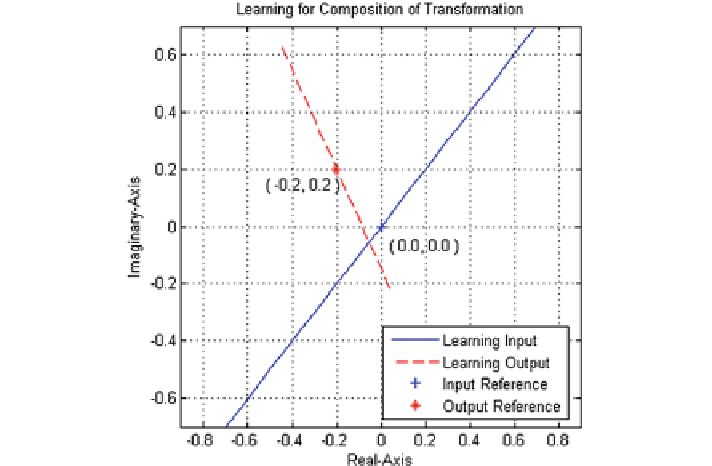
Fig. 5.1 Learning patterns for analysis, mapping shows scaling by factor ʱ , an angle of rotation ˄
and a displacement by distance ʲ in the direction of ˃

various simulations examples have been presented here for learning and generaliza-
tion of mapping . In all examples, this chapter has considered a 2-M-2 network,

where M is the number of proposed neurons in a hidden layer. A set of points in the
first input lie on locus of a input curve and second input is the reference point of
input curve. Similarly, the first output neuron gives the locus of transformed curve
and second output is its reference point. The transformations of different curves are
graphically shown in various figures of this section. Black color represents the in-
put test figure, desired output is shown by doted Blue color, and actual results are
shown in Red color. Different examples presented in this section for linear and bi-
linear transformations are significant in performance analysis of novel neurons in a
complex domain.

5.2.1 Linear Transformation

In the present context, the linear mapping is described as a particular case of the
conformal mapping (bilinear transformation). If

( z ) is an arbitrary bilinear trans-

formation [refer to Eq. ( 5.1 )] and c reduces to linear transformation

(composition of Scaling, Rotation, and Translation ) of the form:

= 0, then ( z )

1 ( z ) = az + b (5.2)