Higher-Order Computational Model for Novel Neurons - High Dimensional Neurocomputing: Growth, Appraisal and Applications - page 99

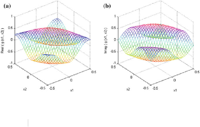
Fig. 4.2 2D Gabor function; a real part and b imaginary part

Table 4.4 Comparison of training and testing performance for 2D Gabor Function
C MLP

C RPN ( d = 0 . 96) C RSS C RSP

Algorithm C BP C RPROP C BP C RPROP C BP C RPROP C BP C RPROP

Network 2-10-1 2-10-1 2-10-1 2-10-1 2-5-1 2-5-1 2-5-1 2-5-1

Parameters 41 41 41 41 41 41 41 41

MSE 0 . 0018 0 . 00088 0 . 0026 0 . 00091 0 . 001 0 . 00097 0 . 00069 0 . 0004

(training)
MSE 0 . 0039 0 . 0016 0 . 0048 0 . 0017 0 . 0019 0 . 00099 0 . 0011 0 . 00062

(testing)
Correlation 0 . 9816 0 . 9913 0 . 9886 0 . 9958 0 . 9954 0 . 9976 0 . 9978 0 . 9979

Error 0 . 0039 0 . 0021 0 . 0046 0 . 0017 0 . 0019 0 . 00079 0 . 0011 0 . 00063

variance
AIC − 6.18 − 6.73 − 5.78 − 6.82 − 6.67 − 7.32 − 7.27 − 7.76

Average 9,000 2,000 9,000 2,000 9,000 2,000 9,000 2,000

epochs

test set. For comparison, we tried the approximation of above function with different
networks using two training algorithms viz C BP ( 01) and C RPROP μ − = ʷ = 0 .

1 . After experimenting
with different numbers of hidden neurons and training epochs, the best result is
reported in Table 4.4 . In order to graphically visualize the 2-D Gabor function, the
real and imaginary part of different network's outputs are shown in Fig. 4.3 . Results
in Table 4.4 clearly demonstrate that the C RSP network with C RPROP perform best
with least error variance and testing error in only 2000 epochs, keeping same number
of learning parameters.

,μ + 10 ( − 6 ) ,ʔ max

0 . 5 = 1 . 2 ,ʔ min = = 0 . 1 ,ʔ 0 = 0 .