Environmental Engineering Reference
In-Depth Information
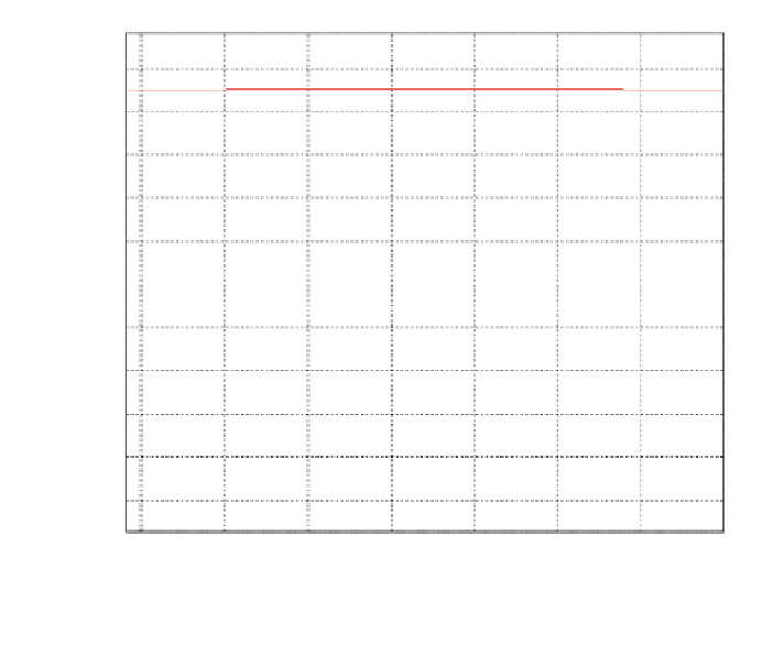
Nichols plot
50
0.001
40
0.005
30
0.01
20
0.05
10
0.1
0
0.3
-10
0.5
0.7
1
-20
1.1
-30
1.5
1.3
L0
-40
2
-50
3
-350
-300
-250
-200
-150
-100
-50
Open-loop phase (deg)
Fig. 14.18 QFT
bounds
and
controller
loop-shaping
for
L
0
(s) = P
0
(s)G
p
(s)c
2
c
1
= [X
rs
(s)/
b
di
(s)]
0
G
p
(s)c
2
c
1
machine at maximum C
p
. This is usually performed by controlling the electrical
torque T
g
and pitch angle b.
The electrical torque T
g
is manipulated in Regions 1 and 2 (below rated,
Fig.
14.10
) in order to get a maximum aerodynamic efficiency C
p
. This strategy
aims to keep optimal the relation between wind speed v
1
and rotor speed X
r
as long
as possible—see k
opt
in Fig.
14.11
a. To do so, the rotor speed X
r
is modified by
changing the electrical torque T
g
, opposite to the wind torque T
r
, to follow the
wind speed changes, and then keep k = k
opt
.
From Eq. (
14.7
), the aerodynamic torque T
r
on the rotor is,
T
r
ð
t
Þ¼
0
:
5 q AC
p
ð
t
Þ
v
1
ð
t
Þ
3
.
X
r
ð
t
Þ
ð
14
:
43
Þ
Now, neglecting mechanical losses in the shaft, the resulting demanded elec-
trical torque T
gd
that maximizes the power capture at every wind speed is:
T
gd
ð
t
Þ¼
K
a
X
r
ð
t
Þ
2
ð
14
:
44
Þ