Environmental Engineering Reference
In-Depth Information
Normal
Faulty
0.1
0.1
0.09
0.09
0.08
0.08
0.07
0.07
0.06
0.06
0.05
0.05
0.04
0.04
0.03
0.03
0.02
0.02
0.01
0.01
0
0
−15
−10
−5
0
5
10
15
−15
−10
−5
0
5
10
15
2
Ω
g
dt
d
2
Ω
g
dt
d
2
2
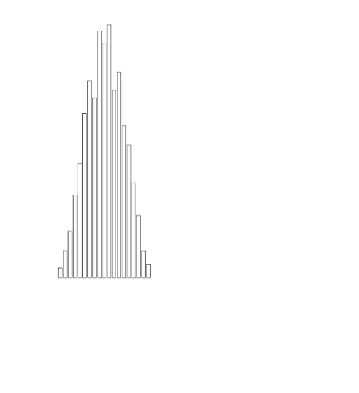
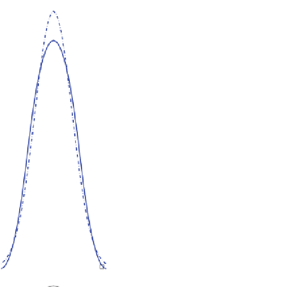
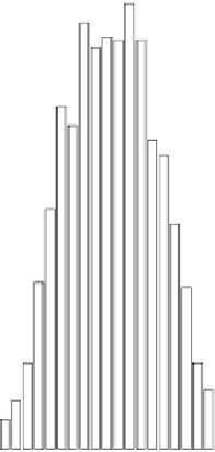
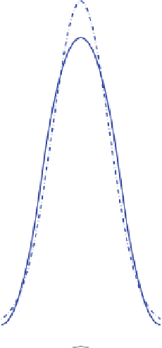
Fig. 10.3 Histogram of the estimated derivative of the generator speed; dashed line, pdf of the
normal distribution N
ð
0
;
q
2
=
2
Þ
; solid line, theoretical pdf of r(k) for uniform white noises
U
ð
q
;
0
Þ
. Left normal healthy condition, q
¼
q
h
¼
60
N
p
T
sc
, Right presence of excessive noise, q
¼
60
ð
1
g
Þ
N
p
T
sc
q
f
¼
where g
¼
10%
To generate fault indicators, the unknown quantity x has to be eliminated from
Eq.
10.22
. To this end, let us consider a full row rank matrix N
C
such that
N
C
C
¼
0. Thus the rows of N
C
span the left null space of matrix C. Multiplying
Eq.
10.22
on the left by N
C
yields:
N
C
y
ð
k
Þ¼
N
C
v
ð
k
Þþ
N
C
f
ð
k
Þ
ð
10
:
23
Þ
Let us set
r
ð
k
Þ
N
C
y
ð
k
Þ
ð
10
:
24
Þ