Environmental Engineering Reference
In-Depth Information
m
3
, in SolidWorks for
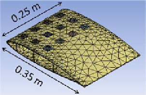
Created blade geometry, with a volume of 5
:
33
10
4
Fig. 8.14
computational analysis
Leading Edge
Thermocouple
For model validation
Fig. 8.15
Location
of
a
temperature
sensor
installed
for
experimental
validation
of
the
computational ANSYS model in an aligned heater layout
the resistors as a function of time created by a PID control to increase the initial
temperature of the blade from 24.9 C to about 30 C. Then, a fifth-order poly-
nomial curve, shown in Fig.
8.16
, was fit to the input voltage using a least squares
curve fitting method. Using this fitted input voltage, the generated heat flux from
each resistor (q (W/m
2
)) is calculated as
2
v
v
max
q
¼
q
max
ð
8
:
3
Þ
where q
max
is the maximum resistor heat flux (W/m
2
) at maximum applied voltage,
v is the input voltage to the resistors (volts), and v
max
is the DC input voltage to the
resistor at maximum power (volts).
The calculated input heat flux was later applied to the heater network in the
ANSYS model. This experiment was done under a natural air convection condi-
tion, with no forced wind velocity to the blade. This natural convection is caused
by buoyancy forces due to density differences caused by temperature variations in
the air. The natural convective heat transfer coefficient of air is in the range
h = 5-25 W/(m
2
C), and the range of the thermal conductivity for a typical
composite material is K = 0.2-1 W/(m
C). Assuming natural convection on the