Information Technology Reference
In-Depth Information
a
b
3
2
2
1
1
0
0
5
10
15
20
0
time
5
−1
0
0.2
0.4
0.6
0.8
1
1.2
1.4
1.6
1.8
0
x
1
−x
*
4
−5
0
5
10
15
20
2
time
5
0
0
−2
−4
−5
0
0.5
1
1.5
2
2.5
0
5
10
15
20
−0.5
time
x
2
−x
*
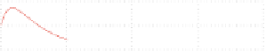
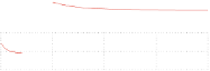
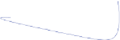
Fig. 3.4
The second fixed point of the circadian oscillator is stable for feedback gain value
c
2
2Œ60:2; 50:2:(
a
) diagrams of the state variables, (
b
) phase diagrams
a
b
2.8
1.4
2.6
1.2
2.4
1
0
0.02
0.04
0.06
0.08
0.1
0.12
0.14
0.16
2.2
time
3
2
1
1.05
1.1
1.15
1.2
1.25
1.3
1.35
1.4
*
x
1
−x
1
2.5
6
2
0
0.02
0.04
0.06
0.08
0.1
0.12
0.14
0.16
time
5
6
4
4
3
2
2
2.1
2.2
2.3
2.4
2.5
2.6
2.7
2.8
0
0.02
0.04
0.06
0.08
0.1
0.12
0.14
0.16
*
x
2
−x
2
time
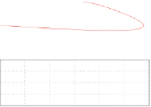
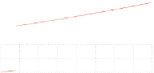
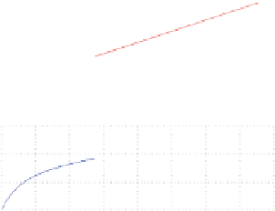
Fig. 3.5
The second fixed point of the circadian oscillator is unstable one for feedback gain value
c
2
2Œ270:2; 260:2:(
a
) diagrams of the state variables, (
b
) phase diagrams
the roots of the characteristic polynomial that is associated with the Jacobian of the
system are
1
D29:49,
2
D1:52, and
3
D0:42, which means that the
fixed point is a stable one. In the second case, that is for c
2
D265 the roots of the
characteristics polynomial became
1
D 59:5,
2
D2:21, and
3
D0:65 which
means that the fixed point is an unstable one. The associated results are depicted in
Figs.
3.4
and
3.5
.
3.8
Conclusions
The chapter has studied bifurcations in biological models, such as circadian cells.
It has been shown that the stages for analyzing the stability features of the fixed
points that lie on bifurcation branches comprise (i) the computation of fixed points
as functions of the bifurcation parameter and (ii) the evaluation of the type of