Information Technology Reference
In-Depth Information
a
b
3
2
1.5
2.5
1
2
0.5
0
1.5
0
5
10
15
20
time
1
3
2
0.5
1
0
0
−0.5
−1
0
0.2
0.4
0.6
0.8
1
1.2
1.4
1.6
1.8
0
5
10
15
20
x
1
−x
*
time
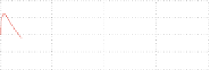
Fig. 3.2
The fixed point of the FitzHugh-Nagumo neuron is a stable one: (
a
) diagrams of the state
variables, (
b
) phase diagrams
a
b
20
20
15
10
10
0
0
5
10
15
20
5
time
20
0
0
2
4
6
8
10
12
*
x
1
10
1
15
0
0
5
10
15
20
time
10
20
5
10
0
0
0
5
10
15
20
0
5
10
15
20
*
time
x
2
2
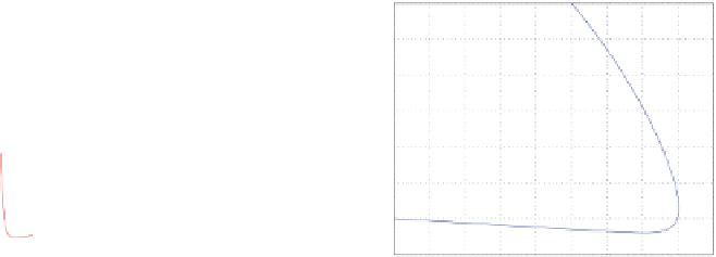
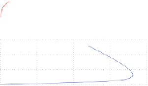
Fig. 3.3
The first fixed point of the circadian oscillator becomes a stable one for parameter
K
d
2Œ0:3;0:9:(
a
) diagrams of the state variables, (
b
) phase diagrams
was an uncertain parameter. It was assumed that the Michaelis constant parameter
varies within intervals, that was K
d
2Œ0:4;0:9 and based on this interval the ranges
of variation of the Jacobian matrix of the model computed at the fixed point
.x
;
1
;x
;
2
;x
;
2
/ D .0;0;0/were found. By applying Kharitonov's theorem it was
possible to show that conditions about the stability of the fixed point were satisfied.
The associated results are depicted in Fig.
3.3
.
Moreover, the case of state feedback was considered in the form K
s
D c
2
x
2
and
using parameter c
2
as feedback gain. The variation range of c
2
was taken to be the
interval Œ60:2; 50:2 and based on this the ranges of variation of the coefficient
of the characteristic polynomial of the system's Jacobian matrix were computed.
Stability analysis followed, using Kharitonov's theorem. First, it was shown that by
choosing 60:2 < c
2
< 50:2 e.g. c
2
D55 then the fixed point .x
;
1
;x
;
2
;x
;
3
/
remained stable.
Next, it was shown that by setting 270:2 < c
2
< 260:2 e.g. c
2
D265
the fixed point became unstable. Indeed in the first case, that is when c
2
D55