Computer Vision Analysis of a Melting Interface Problem with Natural Convection - Visual Computing: Scientific Visualization and Imaging Systems - page 210

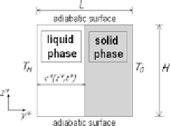
Fig. 12.1 Physical problem
at time t* = 0

Based on the previous hypothesis, the governing equations used in the non-
rectangular liquid domain can be written in their dimensionless form as following:

r V ¼ 0 ð 12 : 3 Þ

q ð T Þ q ref
q ref

k

gH 3
t 2

ð V rÞ V ¼ r 2 V r P+

ð 12 : 4 Þ

Pr r 2 h

( V rÞ h ¼ 1 ð 12 : 5 Þ

The dimensionless velocity vector V is given by: V ¼ V ð Þ= t, where t is the
kinematic viscosity. The dimensionless temperature is given by h ¼ T T av ð Þ= DT ,

where T av is the average temperature given by T av ¼ T H þ T Fu ð Þ= 2. T is the
dimensional temperature, and DT ¼ T H T Fus . The Prandtl number is given by
Pr = t/a, and a is the thermal diffusivity. P is the dimensionless pressure, given by
P ¼ P ðÞ H 2 ; q ref is the reference density (equal to the average density of the
interval imposed by the temperature of the walls) and k is the unitary vector in the
vertical direction. At the moving interface, the energy balance equation is given by:

r h n ¼ o c
os

ð 12 : 6 Þ

The t erm oc = o ð Þ represents the local velocity of the melting front along the
vector n, normal to the interface and s = Ste 9 Fo, with Stefan number given by
Ste = (c p DT)/L F , where c p is the specific heat and L F the latent heat. Fo is the
Fourier number.

12.2.1.1 Density Approximation in the Buoyancy Term

As mentioned earlier, for fluids that reach an extreme density value at a specific
temperature, it is not suitable to assume the hypothesis that the density varies
linearly with temperature. Contrary to the linear estimate that predicts a unicellular
flow, the maximum density formulation predicts a bicellular flow. As for water, the