Probabilistic Distance Clustering: Algorithm and Applications - Clustering Challenges in Biological Network - page 43

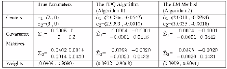
Table 2.1. A comparison of methods for the data of Example 2.1

Table 2.2. A comparison of methods for the data of Example 2.5
True Parameters The PDQ Algorithm The EM Method

(Algorithm 1) (Algorithm 2)

Centers c 1 =(0,0) c 1 =(0.0023 ,-0.0022) c 1 =(0.5429 ,-0.0714)

c 2 =(1,0) c 2 =(1.0080 , 0.0063) c 2 =(1.0603 , 0.02451)

Weights (0.0476 , 0.9524) (0.0534 , 0.9466) (0.1851 , 0.8149)

(d) The number of iterations depends also on the initial estimates, the better
the estimates, the fewer iterations will be required. In our PDQ code
the initial solutions can be specified, or are randomly chosen. The EM
program gets its initial solution from its K -means preprocessor.

Example 2.4. Algorithms 1 and 2 were applied to the data of Example 2.1. Both
algorithms give good estimates of the true parameters, see Table 2.1. The com-
parison of running time and iterations is inconclusive, see Table 2.4.

Example 2.5. Consider the data set shown in Fig. 2.3. The points of the right
cluster were generated using a radially symmetric distribution function Prob

{ x −

µ 2 ≤ µ 2 =(1 , 0),and

the smaller cluster on the left was similarly generated in a circle of diameter 0.1
centered at (0 , 0). The ratio of sizes is 1:20.

r } =(4 / 3) r in a circle of diameter 1.5 centered at

As shown in Table 2.2 and Fig. 2.4(b), the EM Method gives bad estimates of
the left center, and of the weights. The estimates provided by the PDQ Algorithm
are better, see Fig. 2.4(a).
The EM Method also took long time, see Table 2.4. In repeated trials, it did
not work for =0 . 1, and sometimes for =0 . 01.

Example 2.6. Consider the data set shown in Fig. 2.5. It consists of three clusters
of equal size, 200 points each, generated from Normal distributions N ( µ i , Σ i ),