Biology Reference
In-Depth Information
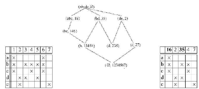
Fig. 8.2.
(a) A context.
(b) The corresponding concept lattice.
(c) Reduced cross-table of
Child
(
abcde, ∅
) of the context.
level manner. More specifically, for a concept
C
=(
obj
(
X
)
,X
),wefirst com-
pute all its children
Child
(
C
). Then we dynamically update the adjacency lists by
representing the attributes in each child of
C
with one single element. We then
use these condensed adjacency lists to process each child of
C
. That is, instead
of using the global adjacency lists, when processing (
obj
(
XS
)
,XS
),weusethe
condensed adjacency lists of its parent. It takes
O
(
S∈
AttrChild(
X
)
|
obj
(
XS
)
|
)
for
C
to generate its condensed adjacency lists
cnbr
() (see Algorithm 8.3 in
the Appendix for the pseudo-code).
And the time for the procedure S
PROUT
is
O
(
a∈
obj(
X
)
|
cnbr
(
a
)
) (see Algorithm 8.2 in the Appendix for the pseudo-
code). Notice that
a∈
obj(
X
)
|
cnbr
(
a
)
|
>
S∈
AttrChild(
X
)
|
obj
(
XS
)
, the time
for updating the adjacency lists is subsumed by the time required for procedure
S
PROUT
. Therefore, our new running time is
O
(
a∈
obj(
X
)
|
cnbr
(
a
)
|
|
) for each
concept (
obj
(
X
)
,X
). See Algorithm 8.4 in the Appendix for the pseudo-code
and Fig. 8.3 for a step-by-step illustration of the algorithm.
|
8.5. Variants of the Algorithm
For some applications, one is not interested in the entire concept lattice. In the
following, we will describe how to modify our algorithm to solve two special
cases: enumerating all concepts only and constructing a frequent closed itemset
lattice.


Search WWH ::

Custom Search