Information Technology Reference
In-Depth Information
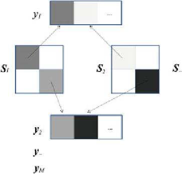
Fig. 8.1
Graphical illustration of the construction of the source energy pro
le vectors y
m
in different representation spaces; applying to (1) any invertible and linearity-pre-
serving transform T leads to
Tvð
t
Þ
½
¼
AT sð
t
Þ
½
;
which preserves the mixing model. Then, solving source separation in the trans-
formed space still provides estimation of the matrix
A
or of its inverse
B
, which can
be used directly in Eq. (
8.2
) for recovering the source
(
t
) in the initial space. For
example, the transform T may be a discrete Fourier transform, a time
s
-
frequency
transform such as the Wigner
Ville transform or a wavelet transform. AJDC can be
easily and conveniently transposed in the frequency domain, thence in the time
-
-
frequency domain, whether we perform the frequency expansion for several time
segments.
It is important to consider that the number of matrices should be high enough to
help non-collinearity of source energy pro
-
les. One may want to have at least as
many matrices in the diagonalization set as sources to be estimated. On the other
hand, one should not try to increase the number of matrices inde
nitely to the
detriment of the goodness of their estimation, i.e., selecting too many discrete
frequencies or blocks of data that are too shorts. In summary, the key for succeeding
with BSS by AJDC is the de
nition of an adequate size and content of the diag-
onalization set; it should include matrices estimated on data as homogeneous as
possible for each matrix, with enough samples to allow a proper estimation, in
frequency region and time blocks when the signal-to-noise ratio is high and with a
high probability to uncover unique source energy pro
les.