Information Technology Reference
In-Depth Information
(a)
(b)
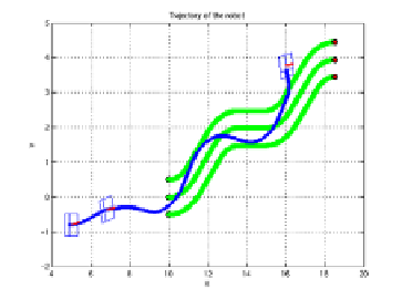
Fig. 15.3
(a) Trajectory of the robot; and (b) visual features evolution
454
m
and
d
max
= 8
m
in (15.1). At the expected
final position, the visual features in the camera image plane must reach the values:
Y
1
= 0
camera is given by taking
d
min
= 2
.
2,
Y
2
= 0, and
Y
3
=
.
−
.
0
2. To guarantee the visibility of the target, the co-
.
efficient
β
wasfixedto0
4. The bounds on the camera velocity and acceleration
are
u
1
=
110
1
,and
u
0
=
115
. By applying the proposed control scheme
with the MATLAB
.
LMI Control Toolbox we obtained the following value for the
control gain
K
:
⎡
⎤
−
505
1392
.
8
−
507
.
8
−
6
.
50
.
18
.
6
⎣
⎦
.
K
=
−
814
35
.
1
784
.
80
.
1
−
12
.
50
.
1
−
937
.
5
−
161
.
2
−
973
.
58
.
60
.
1
−
72
.
8
Figure 15.3 represents the robot trajectory and the evolution of the visual features.
As a result, the target is correctly tracked by the robot despite the uncertainties on
the target-points depth and the unknown value of the target velocity. Finally, when
the target stops, the robot succeeds in stabilizing the camera in front of it, at the
expected relative configuration. The velocities of the robot and the kinematic screw
of the camera are described in Figure 15.4. One can see in Figure 15.5 that the
second components saturate during the very beginning of the task.
15.5.0.2
Application 2
The second application concerns the sequencing of two navigation tasks. The ob-
jective is to show the interest of the control approach to guarantee the satisfaction
of constraints during the transition between tasks, whereas the switching of task-
function may induce a strong variation of velocity. In the first task, the robot has
to follow a wall by using its proximetric sensors and odometry. The second task is
a visual servoing tasks which consists in driving the robot in order to position its
camera in front of a fixed target.

Search WWH ::

Custom Search