Information Technology Reference
In-Depth Information
a
11
a
12
a
13
a
21
a
22
a
23
a
31
a
32
a
33
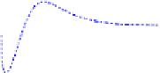
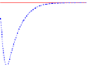
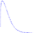
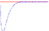
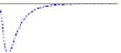
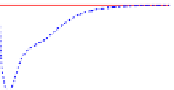
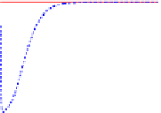
Fig. 8.2
Plain line: the true homography velocity A. Dashed line the observed homography
velocity
A
Now let us set
C
=[
v
]
×
, the skew-symmetric matrix associated with the vector
v
.
Clearly,
C
∈
sl
(3). Then, it follows from (8.31) and (8.32) that
f
(0)=
2
2
+
1)tr(
C
2
)
λ
C
λ
(
λ
−
2
tr(
v
T
1)tr((
v
×
)
2
)
=
λ
v
×
)+
λ
(
λ
−
×
2
tr((
v
×
)
2
)+
1)tr((
v
×
)
2
)
=
−
λ
λ
(
λ
−
tr((
v
×
)
2
)=2
2
= 2
=
−
λ
λ
v
λ
<
0
.
Therefore, there exists
t
1
>
0 such that for any
t
∈
(0
,
t
1
),
f
(0)+
t f
(0)+
t
2
2
f
(0)
f
(
t
)
≈
/
V
u
+
t
2
2
f
(0)
≈
/
<
V
u
.


Search WWH ::

Custom Search