NUMERICAL INTEGRATION OF DIFFERENTIAL EQUATIONS - Computer Methods for Analysis of Mixed-Mode Switching Circuits - page 69

and

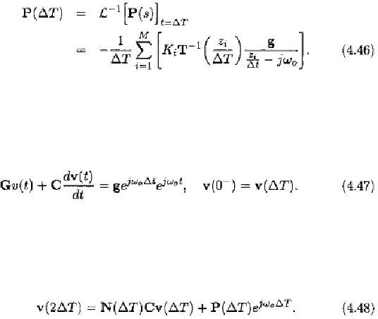
In the second step, we reset the time origin to The input
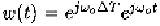
becomes and the initial condition becomes
subsequently. The circuit in the second sub-interval is depicted

by

Following the similar steps as those for the first sub-interval, one can
show that the response of the circuit at the end of the second sub-interval
is given by

Continuing this process, we obtain the response of the circuit at the end
of the

sub-interval

The preceding algorithm computes the response of linear circuits over
a time interval of arbitrary length in a stepping manner, and is hence
termed the stepping algorithm. It is seen from (4.49) that is

the transition matrix of the circuit as it links the present state
to the next state in the absence of the input. on
the other hand, quantifies the response of the circuit when the initial
state is zero, and is hence termed the zero-state vector. The response
of the circuit is completely defined by the transition matrix and the
zero-state vector.