Geoscience Reference
In-Depth Information
Ion displacement distributions
⊥
to
B
0.4
τ
=0
.
0ms
τ
=2
.
0ms
τ
=4
.
0ms
τ
=6
.
0ms
τ
=8
.
0ms
τ
=10
.
0ms
Gaussian
Ion displacement distributions
⊥
to
B
0.3
0.4
0.2
0.2
0.1
0
−2
0
10
8
−3
−2
−1
0
1
2
3
0
6
4
Δ
r
⊥
(
τ
)
/σ
⊥
(
τ
)
2
2
0
Δ
r
⊥
(
τ
)
/σ
⊥
(
τ
)
Time delay [ms]
Ion displacement distributions
to
B
Ion displacement distributions
to
B
τ
=0
.
0ms
τ
=2
.
0ms
τ
=4
.
0ms
τ
=6
.
0ms
τ
=8
.
0ms
τ
=10
.
0ms
Gaussian
0.4
0.3
0.4
0.2
0.2
0.1
0
−2
10
8
0
6
0
4
2
−3
−2
−1
0
1
2
3
2
0
Δ
r
(
τ
)
/σ
(
τ
)
Δ
r
(
τ
)
/σ
(
τ
)
Time delay [ms]
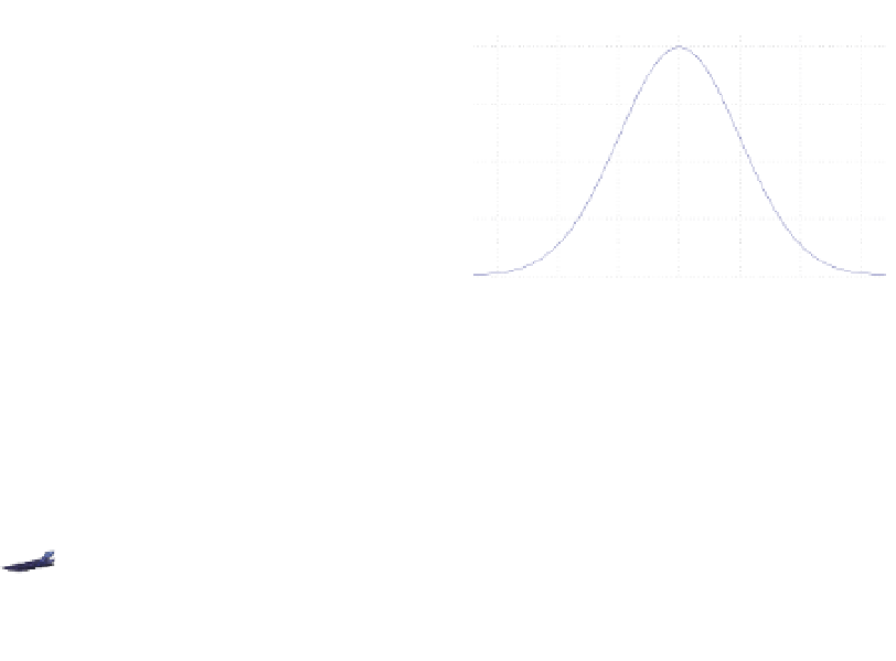
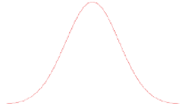
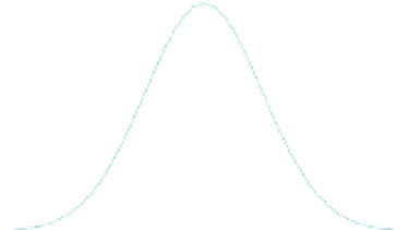
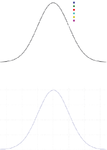
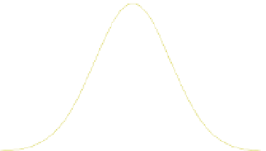
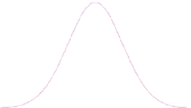
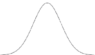
Fig. 5. Probability distributions of the displacements of a test ion in the directions
perpendicular (top panels) and parallel (bottom panels) to the magnetic field. On the left, the
displacement pdf's are displayed as functions of time delay
. On the right, sample cuts of
the pdf's are compared to a Gaussian distribution. Note that all distributions at all time
delays are normalized to unit variance. The displacement axis of each distribution at every
delay
τ
is scaled with the corresponding standard deviation of the simulated displacements
(from Milla & Kudeki, 2011).
τ
of the distributions of the ion displacements in the directions perpendicular and parallel to
the magnetic field. In this case, we have considered an oxygen ion moving in a plasma with
density
N
e
=
10
12
m
−
3
, temperatures
T
e
=
T
i
=
1000 K and magnetic field
B
o
=
25000 nT.
Note that, at every delay
, the distributions have been normalized to unit variance by scaling
the displacement axis of each distribution with the corresponding standard deviation of the
particle displacements. On the left panels, the distributions are displayed as functions of
τ
,
while, on the right panels, sample cuts of these distributions are compared to a Gaussian
pdf showing good agreement. In addition, we can verify that the components of the vector
displacement (i.e.,
τ
r
z
) are mutually uncorrelated.
This analysis implies that ion particle displacements can be represented as jointly Gaussian
Δ
r
components, therefore the single-particle ACF takes the form (e.g., Kudeki & Milla, 2011)
Δ
r
x
,
Δ
r
y
, and
Δ
e
−
1
2
k
2
sin
2
α
Δ
r
2
e
j
k
·
Δ
r
e
−
1
2
k
2
cos
2
α
Δ
r
2
⊥
,
=
×
(45)