Geoscience Reference
In-Depth Information
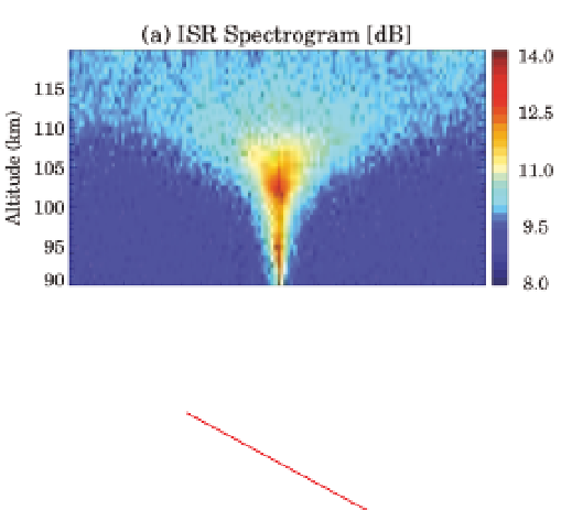
Fig. 2. Collisional D-region spectrograms from Jicamarca Radio Observatory (from Chau &
Kudeki, 2006).
k
B
α
k
⊥
k
Fig. 3. Backscattering geometry in a magnetized ionosphere parametrized by wavevector
components
k
tan
−
1
α
=
(
⊥
)
and
k
and aspect angle
k
/
k
.
⊥
5. Incoherent scatter from a magnetized ionosphere
In a magnetized ionosphere with an ambient magnetic field
B
, it is convenient to express the
scattered wavevector as
, where
b
and
p
are orthogonal unit vectors on
k
-
B
plane which are parallel and perpendicular to
B
, respectively, as depicted in Figure 3. We can
then express the single particle ACF as
bk
k
=
+
pk
⊥
e
j
k
·
Δ
r
e
j
(
k
Δ
r
+
k
⊥
Δ
p
)
=
e
jk
Δ
r
e
jk
⊥
Δ
p
=
×
,
(29)
b
and
where
Δ
r
and
Δ
p
are particle displacements along unit vectors
p
.
Assuming
independent Gaussian random variables
Δ
r
and
Δ
p
, we can then write
e
−
1
2
k
2
Δ
r
2
e
j
k
·
Δ
r
e
−
1
2
k
2
⊥
Δ
p
2
=
×
(30)
in analogy with the non-magnetized case. The assumptions are clearly justified in case of a
collisionless ionosphere (or for intervals
τ
such that
τν
1), in which case
r
2
C
2
2
Δ
=
τ
(31)
and, as shown in Kudeki & Milla (2011),
4
C
2
Ω
p
2
sin
2
Δ
=
(
Ω
τ
/2
)
,
(32)
2