Information Technology Reference
In-Depth Information
A more specific understanding can be obtained from the considerations done in
Section 1.6.3. There, the congruence between the RKHS induced by the mCI kernel,
H
I
, and the RKHS induced by
H
κ
, was utilized to show that the mCI kernel is
inversely related to the variance of the transformed spike times in
κ
,
H
κ
. In this dataset
and for the kernel size utilized, this guaranties that the value of the mCI kernel within
class is always smaller than interclass. This is a reason why in this scenario the first
principal component always suffices to project the data in a way that distinguishes
between spike trains generated each of the templates.
Conventional PCA was also applied to this dataset by binning the spike trains.
Although cross-correlation is an inner product for spike trains and, therefore, the
above algorithm could have been used, for comparison, the conventional approach
was followed [27, 15]. That is, to compute the covariance matrix with each binned
spike train taken as a data vector. This means that the dimensionality of the co-
variance matrix is determined by the number of bins per spike train, which may
be problematic if long spike trains are used or small bin sizes are needed for high
temporal resolution.
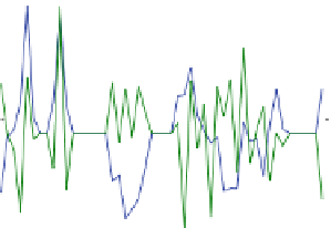
The results of PCA using bin size of 5 ms are shown in Figs. 1.6 and 1.7. The
bin size was chosen to provide a good compromise between temporal resolution and
smoothness of the eigenfunctions (important for interpretability). Comparing these
results the ones using the mCI kernel, the distribution of the eigenvalues is quite
similar and the first eigenfunction does reveal somewhat of the same trend as in
Fig. 1.4. The same is not true for the second eigenfunction, however, which looks
much more “jaggy.” In fact, as Fig. 1.7 shows, in this case the projections along
the first two principal directions are not orthogonal. This means that the covariance
matrix does not fully express the structure of the spike trains. It is noteworthy that
this is not only because the covariance matrix is being estimated with a small num-
ber of data vectors. In fact, even if the binned cross-correlation was utilized directly
in the above algorithm as the inner product the same effect was observed, meaning
that the
binned cross-correlation does not characterize the spike train structure in
90
0.5
first principal component
second principal component
80
0.4
70
0.3
60
0.2
50
0.1
0
40
-0.1
30
20
-0.2
10
-0.3
0
−0.4
0
10
20
30
40
50
0
0.05
0.1
0.15
0.2
0.25
index
time (s)
(a) Eigenvalues in decreasing order.
(b) First two eigenvectors/eigenfunctions.
Fig. 1.6: Eigendecomposition of the binned spike trains covariance matrix.