Information Technology Reference
In-Depth Information
35
1
(a)
(b)
30
0
25
−1
20
−2
15
−3
λ
λ
10
−4
5
−5
0
−6
−7
−5
−10
−8
−15
−9
0
500
1000
1500
2000
2500
3000
3500
4000
0
500
1000
1500
2000
2500
3000
3500
4000
n
n
1
0.4
(c)
(d)
0.3
0.5
0.2
0.1
0
λ
0
λ
−0.5
−0.1
−0.2
−1
−0.3
−0.4
−1.5
−0.5
−2
−0.6
0
500
1000
1500
2000
2500
3000
3500
4000
0
1000
2000
3000
5000
6000
4000
n
n
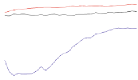
Fig. 16.3: Convergence of the spectrum of Lyapunov exponents for (
a
) the Lorenz
attractor, (
b
)Rossler attractor, (
c
)Henon map, and (
d
)theHenon-Heiles system.
The graphs show the results of the algorithm described in Section 16.2.
16.5.2 Sensitivity Analysis
Two parameters, namely the evolution time
, have been
chosen for further investigation for robustness. We mentioned in Section 2.2.2 that
τ
Δ
t
and the time delay
τ
is determined as the lag which gives us the first minimum for the mutual average
information for our observed data. Figure 16.4 shows how the spectrum of Lyapunov
2
5
0
0
−2
−5
−4
λ
λ
−6
−10
−8
−15
−10
−20
−12
0
5
10
15
20
25
30
0
5
10
15
20
25
30
35
40
τ
Δt
(a)
(b)
Fig. 16.4: The Lyapunov exponents as a function of (
a
)
τ
and (
b
)
Δ
t
for the Lorenz
attractor.