Information Technology Reference
In-Depth Information
100
90
80
70
60
50
40
30
20
10
0
1
2
3
4
5
6
7
8
9
10
Dimension
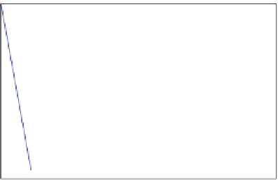
Fig. 16.1: The percentage of false nearest neighbors for 10,000 data points from the
Lorenz equations (see Section 2.2.2). The data were output at
Δ
t
=
0
.
01 during the
integration. A time lag
12, which is the location of the first minimum
in the average mutual information for this system, was used in forming the time-
delayed vectors.
τ
=
12
Δ
t
=
0
.
From the point of view of the mathematics of the embedding process it does not
matter whether one uses the minimum embedding dimension
d
E
or any
d
d
E
, since
once the attractor is unfolded, the theorem's work is done. For a physicist the story is
quite different. Working in any dimension larger than the minimum required by the
data leads to excessive computation when investigating the Lyapunov exponents.
It also enhances the problem of contamination by roundoff or instrumental error
since this noise will populate and dominate the additional
d
≥
d
E
dimensions of
the embedding space where no dynamics is operating. We should add that in going
through the data set and determining which points are near neighbors of the point
y
−
we use the sorting method of a
k
-dimensional tree to reduce the computation
time from
(
n
)
n
2
O
(
)
O
(
N
log
10
(
))
to
N
.
16.4 Models Used in the Computational Experiments
We evaluate the algorithm performance using the signals simulated from four
well-known
dynamical
mathematical
models:
Lorenz,
R ossler,
Henon,
and
Henon-Heilers. Brief descriptions of the models are given below.
16.4.1 Lorenz Attractor
We begin our study of Lyapunov exponents with the Lorenz equations:
x
=
σ
(
y
−
x
)
,
y
=
Rx
−
y
−
xz
,
z
=
xy
−
bz
.