Discovering Image Similarities.Tolerance Near Set Approach - Rough Fuzzy Image Analysis: Foundations and Methodologies - page 237

where sup and inf refer to the supremum and infimum, and d(x, y) is the distance metric
(in this case it is the l 2 norm). The Hausdorff distance is given graphically in Fig. 12.1a.
In this case, the distance from the x∈X to every element of set Y is determined, and
the shortest distance is selected as the infimum. This process is repeated for every x∈X
and the largest distance (supremum) is selected as the Hausdorff distance of the set X to
the set Y . Finally, this process is repeated for the set Y because the two distances will not
necessarily be the same. For example, the Hausdorff distance of the set X to the set Y would
be the distance from the lowercase letters in Fig. 12.1a, but the result would be smaller for
the distance of the set Y to the set X. The method of applying the Hausdorff distance

X Y

X

Y

y

x

y

x

x

x

y

x

x y

x

y

y

x

x

y

y

x

Z = X U Y
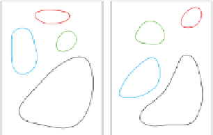
(12.1b) Image Correspondence Prob-
lem

(12.1a) Hausdorff distance

FIGURE 12.1: Graphical Interpretations

to the image correspondence problem is the same as that described in Section 12.3.3. To
reiterate, consider Fig. 12.1b where each rectangle represents a set of subimages (obtained
by partitioning the original images X and Y ) and the coloured areas represent some of the
obtained tolerance classes. The tolerance relation covers both images, but not all the classes
are shown in the interest of clarity. Note, the tolerance classes are created based on the
feature values of the subimages, and consequently, do not need to be situated geographically
near each other (as shown in Fig. 12.1b). In the case of the tNM measure, the idea is that
similar images should produce tolerance classes with similar cardinalities. Consequently, we
are comparing the cardinalities of the portion of a tolerance class belonging to set X with
the portion of the tolerance class belonging to set Y (represented in Fig. 12.1b as sets with
the same colour). In contrast, the Hausdorff distance measures the distance between sets in
some metric space. As a result, we measure distance in the feature space between the portion
of a tolerance class belonging to set X with the portion of a tolerance class belonging to set
Y (again, represented as a sets with the same colour). Here, the idea is that images that are
similar should have tolerance classes are close to each other (in the Hausdorff sense) in the
feature space. As a result, low Hausdorff distances are desirable. Finally, it is important to
note, one may be inclined to intuitively think the Hausdorff distance should always be zero.
However, this is not the case because we are dealing with tolerance where the feature values
are similar, but not the same.

12.4 Illustration: Image Nearness Measures with Microfossil

Images