Image Processing Reference
In-Depth Information
where
g
X
(
x
)and
g
Y
(
y
) are the (average) gray level values of (subimages) pixels
x ∈ X
and
y ∈ Y
.
{b
1
,b
2
, ..., b
N
b
}
are the bins in calculating the histograms of
g
X
(
x
)and
g
Y
(
y
)and
CH
g
X
(
b
j
)and
CH
g
Y
(
b
j
) are cumulative distribution functions
(empirical histograms).
Example 8.7
Sample images and their tolerance classes are shown in Figure 8.12. The number of
overlapping tolerance classes at each subimage,
ω
X
(
x
)) (or
ω
Y
(
y
)) is plotted versus
the index of subimage,
)areshown
in Figure 8.11. TOD and tNM nearness measures are shown in table 8.2 for different
values of
x
(or
y
). The empirical CDFs for
ω
X
(
x
)and
ω
Y
(
y
p × p
subimage size (
p
=10
,
20) and epsilon (
ε
=0
.
01
,
0
.
05
,
0
.
1
,
0
.
2).
B
B
{φ
}
Different sets (
B
1
and
2
) of probe function have been used.
1
=
and
1
B
2
=
φ
2
represent
the entropy of subimage. HSM measure is also calculated using the gray level values
of all the pixels in each image using equation 8.28. #Tol-X and #Tol-Y represent
the number of tolerance classes for images X and Y, respectively. The results are
shown in table 8.2 and plotted in figure 8.13.
{φ
1
,φ
2
}
where
φ
1
represents average gray value of a subimage and
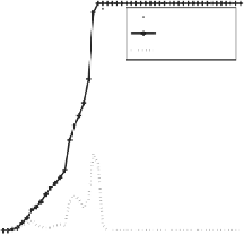
Empirical histograms / Distributions
Cumulative histograms / CDFs
200
1
1st Histogram H
X
(b
i
)
2nd Histogram H
Y
(b
i
)
1st CDF CH
X
(b
i
)
2nd CDF CH
Y
(b
i
)
|CH
X
Ŧ CH
Y
|
180
0.9
160
0.8
140
0.7
120
0.6
100
0.5
80
0.4
60
0.3
40
0.2
20
0.1
0
0
0
0.2
0.4
0.6
0.8
1
0
0.2
0.4
0.6
0.8
1
Histogram Bins: b
i
Histogram Bins: b
i
FIGURE 8.11: CDF of the number of overlaps between tolerance classes for
ω
X
(
x
)
and
ω
Y
(
y
)
Similarity between groups of conceptually different images
The similarity measures discussed in section 8.3.1, can be calculated for each pair of
images in an image database to reveal structures in the set of images and possibly
be used for clustering or classification of images or image retrieval. In order to


Search WWH ::

Custom Search