Image Processing Reference
In-Depth Information
(7.7a)
(7.7b)
(7.7c)
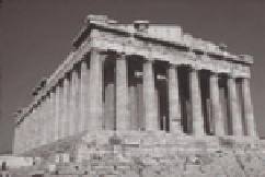
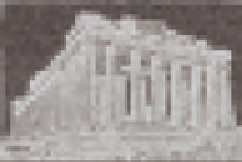
FIGURE 7.7: Example of Shannon's entropy applied to images: (a) Original image (Martin
et al., 2001), (b) Shannon's entropy applied to subimages of size 5×5, and (c) Shannon's
entropy applied to subimages of size 10×10.
P2: lim
p
i
→0
∆I(p
i
) = ∆I(p
i
= 0) = k
,k
> 0 and finite.
1
1
P3: lim
p
i
→1
∆I(p
i
) = ∆I(p
i
= 1) = k
,k
> 0 and finite.
2
2
P4: k
.
P5: With increase in p
i
, ∆I(p
i
) decreases exponentially.
P6: ∆I(p) and H, the entropy, are continuous for 0≤p≤1.
P7: H is maximum when all p
i
's are equal, i.e. H(p
< k
2
1
,...,p
n
)≤H(1/n,..., 1/n).
With these in mind, (Pal and Pal, 1991) defines the gain in information from an event as
∆I(p
i
) = e
(1−p
i
)
,
1
which gives a new measure of entropy as
n
X
p
i
e
(1−p
i
)
.
H =
i=1
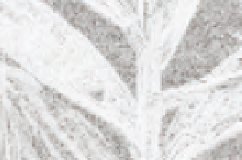
Pal's version of entropy is given in Fig. 7.8. Note, these images were formed by first
converting the original image to greyscale, calculating the entropy for each subimage, and
multiplying this value by 94 (since the maximum of H is e
1−1/256
).
(7.8a)
(7.8b)
(7.8c)
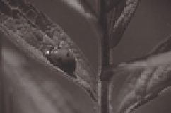
FIGURE 7.8: Example of Pal's entropy applied to images: (a) Original image (Martin
et al., 2001), (b) Pal's entropy applied to subimages of size 5×5, and (c) Pal's entropy
applied to subimages of size 10×10.
7.4.5
Edge based probe functions


Search WWH ::

Custom Search