Environmental Engineering Reference
In-Depth Information
EXAMPLE 3.22
The covariance function of the longitudinal component
of the flow velocity in an open channel can be approxi-
mated by the relation
1
∆
x
m /s
C
11
(
∆
)
=
0 25
.
exp
−
2
2
x
10
0
where Δ
x
is the spatial lag in the flow direction in meters.
If the mean flow velocity is 2 m/s, then estimate the
Lagrangian covariance of the longitudinal velocity fluc-
tuations and the longitudinal diffusion coefficient.
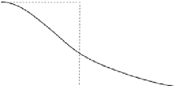
T
11
time lag,
t
Lagrangian time scale
Figure 3.23.
relationship between Lagrangian time scale and
velocity autocorrelation function.
Solution
where
ρ
ij
(
τ
) is the correlation between the velocity fluc-
tuations
v t
i
( )
and
v t
′ +
j
(
τ
, and is given by
According to the frozen turbulence assumption, the
spatial lag, Δ
x
, is related to the time lag,
τ
, by the
relation
′
( )
′
+
(
)
v t v t
τ
i
j
ρ τ
( ) =
(3.215)
ij
σ σ
v
v
i
j
∆
x
= vτ
where
σ
v
i
and
σ
v
j
are the standard deviations of the
velocity components
v
i
and
v
j
, respectively. The relation-
ship between the Lagrangian velocity autocorrelation
function and the Lagrangian time scale is illustrated in
Figure 3.23.
Since the Lagrangian velocity correlation function
ρ
ij
(
τ
) is related to the Lagrangian velocity covariance
function,
C
ij
(
τ
) by
Since
V
= 2 /
, then in this case, Δ
x
= 2
τ
. The Lagrang-
ian covariance of the longitudinal velocity fluctuations
can then be estimated by the relation
m s
2
10
τ
=
C
11
( )
τ
≈
0 25
.
exp
−
0 25
.
exp(
−
0 2
.
τ
)
m /s
2
2
The longitudinal diffusion coefficient is defined by
Equation (3.208) in terms of the Lagrangian covariance
function as
C
ij
( )
τ
=
σ σ ρ τ
( )
(3.216)
v
v
ij
i
j
Combining Equations (3.216), (3.214), and (3.208), the
turbulent diffusion coefficient in a statistically homoge-
neous velocity field can be expressed in terms of the
Lagrangian velocity time scale,
T
ij
, by the relation
∞
∞
∫
∫
( )
ε
=
C
τ τ
d
≈
0 25
.
e
−
0 2
.
τ
d
τ
11
11
0
0
[
]
∞
=
0 25 5
.
−
e
−
0 2
.
τ
0
2
=
1 25
.
m /s
∞
∫
0
( )
ε
=
σ σ
ρ τ τ
d
ij
v
v
ij
i
j
(3.217)
Therefore, the longitudinal diffusion coefficient corre-
sponding to the given Eulerian velocity covariance
function is approximately 1.25 m
2
/s.
=
σ σ
T
v
v
ij
i
j
If the coordinate axes are taken in the principal direc-
tions of the velocity fluctuations,* the nonzero diffusion
coefficient components can be written as
Lagrangian Time Scale.
The Lagrangian time scale,
T
ij
,
is a measure of the time lag,
τ
, over which the Lagrang-
ian velocity fluctuations
σ
2
i
T
,
i
,
otherwise
=
1 3
ii
v
ε
=
(3.218)
ii
0
j
( τ
are signifi-
cantly correlated. The Lagrangian time scale is formally
defined by the relation
v t
i
( )
and
v t
′ +
or in the more common Cartesian forms
*
When the coordinate axes are in the principal directions of the
velocity fluctuations, the velocity covariance matrix is diagonal, in
which case cross-covariances are equal to zero.
∞
∫
( )
T
=
ρ τ τ
d
(3.214)
ij
ij
0


Search WWH ::

Custom Search