Environmental Engineering Reference
In-Depth Information
1
t
=
t
1
0.8
0.6
x
Vt
0.4
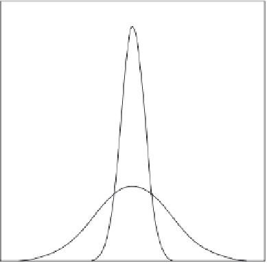
Figure 3.7.
Solution to the one-dimensional advection-
diffusion equation.
0.2
t
=
t
2
in the
x
′ -
t
domain, where
x
′ =
x
−
Vt
. The initial and
boundary conditions corresponding to an instantaneous
release at
x
= 0 and
t
= 0 with boundaries infinitely far
away from the release location are
0
−
4
−
2
0
2
4
x
Figure 3.6.
one-dimensional diffusion.
M
A
(3.63)
under the curve. Note that a
normal
distribution is the
same as a Gaussian distribution, except that the area
under the curve,
A
0
, is equal to unity. Comparing the
fundamental solution of the diffusion equation, Equa-
tion (3.57), with the Gaussian distribution, Equation
(3.58), it is clear that the fundamental solution is Gauss-
ian with the mean and standard deviation given by
c x
(
′
, )
0
=
δ
(
x
′
)
c
(
±∞
, )
t
= 0
(3.64)
where
A
is the area in the
yz
plane over which the con-
taminant is well mixed. The solution to Equation (3.62)
subject to initial and boundary conditions given by
Equations (3.63) and (3.64) is the same as the funda-
mental solution for a stationary fluid, and is therefore
given by
µ= 0
(3.59)
(3.60)
σ= 2
D t
x
M
x
D t
′
2
This result demonstrates that a mass of contaminant
released instantaneously into a stagnant fluid will attain
a concentration distribution that is Gaussian, with the
maximum concentration remaining at the location
where the mass was released, and the standard devia-
tion of the distribution growing in proportion to the
square root of the elapsed time since the release. For
Gaussian distributions, 95% of the area under the curve
falls within ±2
σ
of the mean, and so in the present
context, 95% of the released mass is within
μ
± 2
σ
, As
a consequence, the size of the contaminated region,
L
x
,
is commonly taken as
L
x
= 4
σ
.
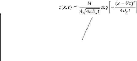
The one-dimensional advection-diffusion equation
in a fluid moving with a constant velocity is given by
c x t
(
, )
=
exp
−
′
(3.65)
4
A
4
π
D t
x
x
which in the
x
-
t
domain is given by
M
(
x Vt
D t
−
)
2
c x t
( , )
=
exp
−
(3.66)
4
A
4
π
D t
x
x
The concentration distribution described by Equation
(3.66) and illustrated in Figure 3.7 describes the mixing
of a tracer released instantaneously into a flowing fluid,
where the tracer undergoes one-dimensional diffusion.
If the fluid is stagnant,
V
= 0, the resulting concentration
distribution is symmetrical around
x
= 0 and is described
by Equation (3.57). If the contaminant undergoes first-
order decay, then, in accordance with the result in Section
3.2.2.2, the concentration distribution is given by
∂
∂
c
t
∂
∂
c
x
∂
∂
c
x
2
(3.61)
+
V
=
D
x
2
where
V
is the fluid velocity in the
x
direction. Equation
(3.61) transforms to
−
kt
2
Me
(
x Vt
D t
−
)
c x t
( , )
=
exp
−
(3.67)
4
A
4
π
D t
x
x
∂
∂
c
t
∂
∂
′
2
c
(3.62)
=
D
x
x
2
where
k
is the first-order decay constant.


Search WWH ::

Custom Search