Environmental Engineering Reference
In-Depth Information
equation plus the initial and boundary conditions for
that particular problem. obviously, there are an infinite
number of solutions to the advection-diffusion equa-
tion, with different solutions corresponding to different
sets of initial and boundary conditions.
There are a few fundamental solutions of the
advection-diffusion equation that constitute the bases
from which numerous other solutions can be derived.
These fundamental solutions generally correspond
to instantaneous releases of a tracer in an infinite
(unbounded) environment with a spatially uniform
velocity field. In accordance with the uniform velocity
field transformation described previously (in Section
3.2.2), these fundamental solutions are derived in a
transformed space where there is only diffusion, with
advection being incorporated by inverse transform of
the diffusion-only fundamental solutions. The inverse
transform typically has the form
concentrations are always equal to zero at
x
= ±∞, the
initial and boundary conditions are given by
M
A
c x
( , )
0 =
δ
( )
x
(3.54)
c
(
±∞
, )
t
= 0
(3.55)
where
A
is the area in the
yz
plane over which the con-
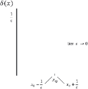
taminant is well mixed, and
δ
(
x
) is the
Dirac delta func-
tion
, which is defined by
∞
x
x
=
≠
0
+∞
∫
δ
( )
x
=
and
δ
( )
x dx
=
1
(3.56)
0
0
−∞
A graph of the Dirac delta function, centered at
x
0
(where
x
0
= 0 in Eq. 3.56), is illustrated in Figure 3.5. The
solution to Equation (3.53), subject to initial and bound-
ary conditions given by Equations (3.54) and (3.55), is
′
=
x
i
and
x
i
are the coordinates in the transformed and
untransformed spaces respectively,
V
i
is the advection
velocity, and
t
is time. The fundamental solutions of the
diffusion equation in one, two, and three dimensions
and example applications are given in the following
sections.
x
x V t
−
, where
′
i
i
i
M
x
D t
2
(3.57)
c x t
( , )
=
exp
−
4
A
4
π
D t
x
x
This result indicates that the concentration distribution
resulting from the instantaneous introduction of a mass
M
is in the form of a Gaussian distribution with a vari-
ance growing with time, as illustrated by a plot of Equa-
tion (3.57) given in Figure 3.6. To verify that the
concentration distribution given by Equation (3.57) is
Gaussian, consider the general equation for a Gaussian
distribution given by
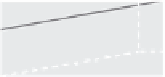
3.3.1 Diffusion in One Dimension
Consider the case where a tracer is distributed uni-
formly in the
y
and
z
directions and diffusion occurs
only in the
x
direction. Such a case is illustrated in
Figure 3.4, where the tracer is completely mixed across
the cross section and any further mixing can occur only
in the longitudinal (
x
) direction. The diffusion equation
is then given by
2
A
1
2
x
µ
σ
−
0
f x
( )
=
exp
−
(3.58)
σ π
2
2
∂
∂
c
t
∂
∂
c
x
(3.53)
=
D
x
where
μ
is the mean of the distribution,
σ
is the standard
deviation of the distribution, and
A
0
is the total area
2
If a tracer of mass
M
is introduced instantaneously at
x
= 0 at time
t
= 0 (well mixed over
y
and
z
), and tracer
tracer mixed across channel
water surface
area = A
z
x
y
x
channel
Figure 3.4.
one-dimensional diffusion.
Figure 3.5.
Dirac delta function.


Search WWH ::

Custom Search