Environmental Engineering Reference
In-Depth Information
The expected value of
Z
is equal to
μ
Z
, which is given
by Equation (10.46) as
EXAMPLE 10.6
A random variable,
X
3
, is defined by the relation
µ
Z
= 0
X
X
/
/
ν
ν
1
1
X
=
3
2
2
10.4.3
F
Distribution
where
X
1
and
X
2
are chi-squared variates with
ν
1
and
ν
2
degrees of freedom, respectively. If
ν
1
= 20 and
ν
2
= 20,
determine the value of
X
3
that is exceeded with 5%
probability. What is the expected value of
X
3
?
If
X
1
and
X
2
are independent chi-squared distributed
random variates with
ν
1
and
ν
2
degrees of freedom,
respectively, then the random variable defined by the
relation
Solution
X
X
/
/
ν
ν
1
1
F
=
(10.47)
2
2
The random variable
X
3
has a
F
distribution with
ν
1
and
ν
2
degrees of freedom. Values of
X
3
with an exceedance
probability of 5% (
α
= 0.05) are given in Appendix C.4
as a function of
ν
1
and
ν
2
. For
ν
1
= 20 and
ν
2
= 20, Appen-
dix C.4 gives
has a probability density function given by
Γ
[(
ν
+
ν
) / )]
2
ν
ν
/
2
ν
ν
/
2
f
(
ν
/ )
2
−
1
(
ν
+
ν
f
)
−
(
ν ν
+
)/
2
1
2
1
1
2
1
2
2
1
1
2
p f
( )
=
,
Γ
(
ν
/
2) (
Γ
ν
/
2)
1
2
X
3
= .
2 12
ν ν
,
,
f
>
0
1
2
(10.48)
The expected value of
X
3
,
µ
X
3
, is given by Equation
(10.49) as
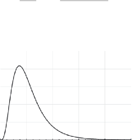
The probability density function
p
(
f
) defines the F
distribution
,* with
ν
1
and
ν
2
degrees of freedom. The
shape of the
F
distribution is illustrated in Figure 10.6.
The mean and variance of the
F
distribution are given
by
ν
ν
20
20 2
1
µ
=
=
= .
1 11
X
3
−
2
−
2
10.5 ESTIMATION OF POPULATION
DISTRIBUTION FROM SAMPLE DATA
ν
ν ν
ν ν
2
(
+
2
)
1
2
1
2
µ
=
,
σ
=
)
(10.49)
F
F
ν
−
2
(
−
2
)(
ν
−
4
2
1
2
2
Analysis of water-quality data is typically a two-step
procedure. In the first step, the sample probability dis-
tribution is compared with a variety of theoretical dis-
tribution functions, and the theoretical distribution
function that best fits the sample probability distribu-
tion is taken as the population distribution. In the
second step, properties of the data are analyzed using
the theoretical population distribution.
The most common methods of estimating population
distributions from measured data are: (1) visually com-
paring the sample probability distribution with various
theoretical distributions and picking the closest distri-
bution that is consistent with the underlying process
generating the sample data; and (2) using hypothesis-
testing methods to assess whether various probability
distributions are consistent with the sample probability
distribution. Hypothesis-testing methods are based on
identifying a statistic that measures the difference
between the sample distribution and the proposed pop-
ulation distribution, and then determining the signifi-
cance level of this statistic. The
significance level
,
α
,
of the statistic is equal to the probability that the
The cumulative
F
distribution is given in Appendix
C.4.
1.0
0.8
0.6
n
1
= 10,
n
2
= 20
0.4
0.2
0.0
0
1
2
3
4
5
f
Figure 10.6.
F
probability distribution.
*
The
F
distribution is named after r.A. Fisher.


Search WWH ::

Custom Search