RIVERS AND STREAMS - Water Quality Engineering in Natural Systems - page 98

This equation was originally derived by Streeter and
Phelps (1925) and later summarized by Phelps (1944)
for studies of pollution in the ohio River. Equation
(4.71) is commonly referred to as the Streeter-Phelps
equation , and a plot of the Streeter-Phelps equation is
commonly referred to as the Streeter-Phelps oxygen sag
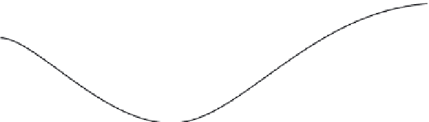
curve . The reason for using the term sag curve is appar-
ent from a plot of the oxygen deficit, D ( x ), as a function
of distance, x , from the source as illustrated in Figure
4.6. According to the Streeter-Phelps equation (Eq.
4.71), oxygen consumption for biodegradation begins
immediately after the waste is discharged, at x = 0, with
the oxygen deficit in the stream increasing from its
initial value of D 0 . Since reaeration is proportional to
the oxygen deficit, the reaeration rate increases as
the oxygen deficit increases, and at some point, the
reaeration rate becomes equal to the rate of oxygen
consumption. This point is called the critical point , x c ,
and beyond the critical point, the reaeration rate
exceeds the rate of oxygen consumption, resulting in a
gradual decline in the oxygen deficit. The critical point,
x c , can be derived from Equation (4.71) by taking
dD / dx = 0, which leads to

dL
dt

= − k L

r

(4.67)

where the reaction rate constant, k r , accounts for both
the bioconsumption of dissolved BoD, k d , and the
removal of BoD by sedimentation, k s , such that
k r = k d + k s as given by Equation (4.58). Integrating
Equation (4.67) gives the BoD as a function of time as

L L = exp ( − k t

r

)

(4.68)

0

where L 0 is the BoD remaining at time t = 0. The time
since release, t , is related to the distance traveled by

x
V

(4.69)

t =

and hence the remaining BoD, L , at a distance x down-
stream of a wastewater discharge is obtained by com-
bining Equations (4.68) and (4.69) to give

x
V

L L =

0 exp

− k (4.70)

r

V k

k

D k ( − k )

The differential equation describing the oxygen deficit
in a river is therefore given by the combination of Equa-
tions (4.66) and (4.70), and the simultaneous solution of
these equations with the boundary condition that
D = D 0 at x = 0 is given by

a 0 a r

ln 1 − k ≠ k

a r

k − k k L

a r r d 0

x

c =

(4.72)

V
k

k
k

D
L

d 0

− k = k

a r

d a 0

and the corresponding critical oxygen deficit, D c , is
given by

k L
k

k x
V

k x
V

−

d 0 r a

exp − exp −

− k

a r

k ≠ k

a r

k x
V

k
k L

k x
V

a

D x ( ) = + D exp −

d r c

D =

0 exp

− (4.73)

0

c

a

k L x
V

k x
V

k x
V

+

a a

exp − D exp − k = k

d 0 0 a r

The location of the critical point and the oxygen con-
centration at that point are of particular interest because (4.71)

saturation concentration

c s

D 0

c 0 D ( x )

D c

c min

critical point

0 x c

downstream distance, x

Figure 4.6. Streeter-Phelps oxygen sag curve.