Geoscience Reference
In-Depth Information
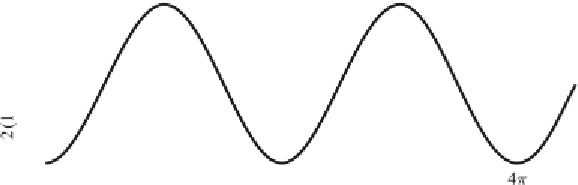
Figure 16.4 The spectral transfer function of the two-point scalar difference
operator.
Thus the difference variance is
φ
d
(
κ
)d
κ
=
2 [1
(c)
2
=
−
cos
(
κ
·
r
)
]
φ(
κ
)d
κ
.
(16.60)
r
)
] of the scalar difference operator
is shown in
Figure 16.4
.
Let's interpret it physically. First, Fourier components
of wavenumber perpendicular to the separation vector
r
have
κ
·
The spectral transfer function 2 [1
−
cos
(
κ
·
r
=
0, so that
cos
(
κ
·
1 and the transfer function is zero; these components are rejected by
the difference filter. More generally, in the small-separation limit
κ
·
r
)
=
0the
two sensors detect essentially the same signal so their difference variance is nearly
zero. Put another way, the difference filter rejects eddies that are much larger than
the separation distance.
As
κ
·
r
→
r
increases from zero the magnitude of the transfer function gradually rises
π
. Here Fourier components
in the
r
direction at the two points are 180 degrees out of phase so they add, not
subtract. This happens again at
κ
·
r
=
(
2
n
−
r
=
1
)π, n
=
2
,
3
,...
The difference array is often used for separations in the inertial range of scales,
where the spectrum
φ(
κ
)
is typically assumed to have its isotropic form
φ(
κ
)
(Chapter 15)
. Let us assume that the separation vector is in the
x
1
-direction. We
can then write
(16.60)
as
∞
cos
(κ
1
r)
]
∞
−∞
φ(κ)dκ
2
dκ
3
dκ
1
(c)
2
=
2 [1
−
−∞
(16.61)
∞
cos
(κ
1
r)
]
F
1
(κ
1
)dκ
1
.
=
2 [1
−
−∞
If the separation vector is in the
x
2
-direction the result is
∞
cos
(κ
2
r)
]
F
2
(κ
2
)dκ
2
,
(c)
2
=
2 [1
−
(16.62)
−∞