Geoscience Reference
In-Depth Information
If we define the mean rate of transfer of variance through wavenumber
κ
from
all smaller wavenumbers as the “cascade rate”
Ca(κ)
, then the net rate of gain of
variance at wavenumber
κ
by such transfer is
Ca(κ)
−
Ca(κ
+
κ)
∂Ca(κ)
∂κ
lim
κ
=−
=
T(κ).
(16.20)
κ
→
0
Then the spectral variance budget
Eq. (16.19)
can be written
∂E
c
(κ)
∂t
∂Ca(κ)
∂κ
2
γκ
2
E
c
(κ).
=
P(κ)
−
−
(16.21)
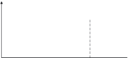
We can briefly explain the behavior of the cascade rate
Ca(κ)
, which is sketched
in
Figure 16.2
.
Integration of the steady-state formof
Eq. (16.21)
over the production
range, from
κ
=
0to
κ
=
κ
end
, say, and using
Eq. (16.4)
gives
κ
end
Ca(κ
end
)
=
P(κ)dκ
=
Pr
=
χ
c
.
(16.22)
0
Thus, in the variance-containing range
Ca(κ)
increases from 0 to
χ
c
.
In the inertial subrange of wavenumbers,
κ
e
κ
d
, the production and
destruction terms in the steady form of the spectral budget
(16.19)
are negligible
so it reduces to
κ
∂Ca(κ)
∂κ
=
0
,
(16.23)
and
Ca(κ)
χ
c
. This is the counterpart of the inertial subrange in the velocity
spectrum; its existence was postulated first by
Obukhov
(
1949
)and
Corrsin
(
1951
).
At yet larger
κ
, in the dissipative range, molecular destruction of scalar variance is
important and the steady spectral variance budget is
=
∂Ca(κ)
∂κ
2
γκ
2
E
c
(κ),
=−
(16.24)
and
Ca(κ)
decreases to zero at large
κ
.
Figure 16.2 The behavior of
Ca(κ)
, the cascade rate of scalar variance.