Neural Networks: An Overview - Neural Networks: Methodology and Applications - page 15

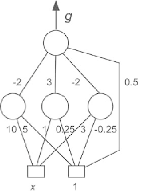
Fig. 1.8. A feedforward neural network with one variable (hence two inputs) and
three hidden neurons. The numbers are the values of the parameters

(see Chap. 2), resulting in the parameters shown on Fig. 1.9(a). Figure 1.9(b)
shows the points of the training set and the output of the network, which
fits the training points with excellent accuracy. Figure 1.9(c) shows the out-
puts of the hidden neurons, whose linear combination with the bias provides
the output of the network. Figure 1.9(d) shows the points of a test set, i.e., a
set of points that were not used for training: outside of the domain of variation
of the variable x within which training was performed ([ 0 . 12 , +0 . 12]), the

approximation performed by the network becomes extremely inaccurate, as
expected. The striking symmetry in the values of the parameters shows that
training has successfully captured the symmetry of the problem (simulation
performed with the NeuroOne TM software suite by NETRAL S.A.).
It should be clear that using a neural network to approximate a single-
variable parabola is overkill, since the parabola has two parameters whereas
the neural network has seven parameters! This example has a didactic charac-
ter insofar as simple one-dimensional graphical representations can be drawn.

−

1.1.4 Feedforward Neural Networks with Supervised Training for
Static Modeling and Discrimination (Classification)

The mathematical properties described in the previous section are the basis
of the applications of feedforward neural networks with supervised training.
However, for all practical purposes, neural networks are scarcely ever used for
uniformly approximating a known function.
In most cases, the engineer is faced with the following problem: a set of
measured variables

x k , k =1to N y p ( x k ),

{ } , and a set of measurements {