Closed-Loop Control Learning - Neural Networks: Methodology and Applications - page 304

11 12 13 14 15

21 22 23 24 25

31 32 33 34 35

41 42 43 44 45

51 52 53 54 55

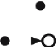
Fig. 5.12. Diagram of labyrinth from Fig. 4.1 with trajectories that are associated
to constant policy GO EASTWARDS

In our simple example, the set of feasible actions is always N, S, E, W
(north, south, east, west) and does not depend on the current state. A dy-
namical system is associated to a given policy. If this policy is stationary,
the dynamical system is autonomous. Thus, in our example, consider the sta-
tionary constant policy GO EASTWARDS , which associates E action to
any current state. State trajectories of the associated dynamical system are

ω 1 = ((12, E), (13, E), (14, E), (15, E), (15, E) ... ) trajectory coming from
initial state 12,
ω 2 = ((21, E), (22, E), (22, E), ... ) trajectory coming from initial state 21,
ω 3 =((24, E), (24, E),...) trajectory coming from initial state 24,
ω 4 = ((32, E), (33, E), (34, E), (35, E),(35) ... ) trajectory coming from initial
state 32, etc.

Those trajectories are shown on Fig. 5.12.
A total cost J is associated to each state-action trajectory. In principle,
it is the sum of the elementary costs of each step of the trajectory. One has
to make a distinction between finite horizon problems and infinite horizon
problems. In finite horizon problems, where the number of steps is fixed in
advance, for instance to N , it is su cient to compute the total cost as the
simple sum of the elementary costs of each step. One can possibly add a
terminal cost function of the final state. For instance, when one considers
“GO EASTWARDS” policy and horizon N = 10, the cost function is J N ,
which takes the following values on the previous trajectories

J N ( ω 1 )=10 , J N ( ω 2 )=10 , J N ( ω 3 )=10 , J N ( ω 4 )=3 − 7 A...

in the case without terminal cost.