Modeling Methodology: Dimension Reduction and Resampling Methods - Neural Networks: Methodology and Applications - page 218

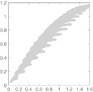
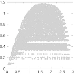
Fig. 3.8. Distribution of distances in the plane ( dy − dx ) for the hemisphere and
sphere

For the nonlinear varieties illustrated by those examples, the projection
must exclude certain points. That is true for the map of the earth obtained
using Mercator's projection. The “western” projection separates the coastlines
of the Bering straits.
In the plane dy

dx , the scatter diagram takes the form of a bell: points
close to each other in the original space ( dx small) will be further apart ( dy
large) in projection space. The bell shape appears clearly for the projection of
the sphere, where an opening separates the points on the large diameter (Fig.
3.5). Checking the projection consists in checking that the bell shape retains
the local topology as far as possible: if two points are close in the reduced
space, they must be close in the original space.

−

3.5.5 Di culties of Curvilinear Component Analysis

Before describing an application, we outline the shortcomings of CCA. The
first problem is that of computation time. The distances between points should
be computed. If the number of points is too great, CCA cannot be applied
directly to the data. A preliminary sampling step is necessary to reduce the
number of examples.
The second problem is related to the use of CCA in on-line mode. Unlike
PCA, reduced components cannot be computed directly. They are obtained
by iterations of gradient descent. Let us describe the CCA procedure. Let
x 0 be a new input; we want to find the corresponding component y 0 .The
algorithm consists in initializing y 0 by the center of gravity of 3 or 4 points y k
that correspond to the points x k closest to x 0 . The projection y 0 is calculated
using the same algorithm: