Modeling with Neural Networks: Principles and Model Design Methodology - Neural Networks: Methodology and Applications - page 181

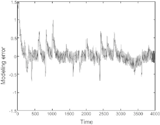
Fig. 2.56. Modeling error on the test set
Since the results are still unsatisfactory (the root mean square error on
the test set is twice the standard deviation of noise), the conjecture that the
right-hand side of the second state equation does not depend on x 1 only, but
also depends on x 2 , must be taken into account. Then a third knowledge-based
neural model may be designed, where the right-hand side of the second state
equation is implemented as a neural network whose inputs are x 1 and x 2 .
That is shown on Fig. 2.57 (with a feedforward network having three hidden
neurons).
Steps 2 et 3 of the design are performed as for the previous model. The
variance of the modeling error being on the order of the noise variance (see
Fig. 2.58), the model can be considered satisfactory.
2.8.1.3 Discretization of a Knowledge-Based Model
The first step of the design of a semiphysical model is the discretization of
the knowledge-based model, which is generally a continuous-time model, in
order to find a discrete-time model whose structure is used for the design of
the recurrent network. The choice of the discretization technique has impor-
tant consequences regarding the stability of the model to be designed. The
discretization of continuous-time differential equations is a basic chapter in
any textbook of numerical analysis; we recall a few basic elements that are
important for the design of a semiphysical model.