Modeling with Neural Networks: Principles and Model Design Methodology - Neural Networks: Methodology and Applications - page 178

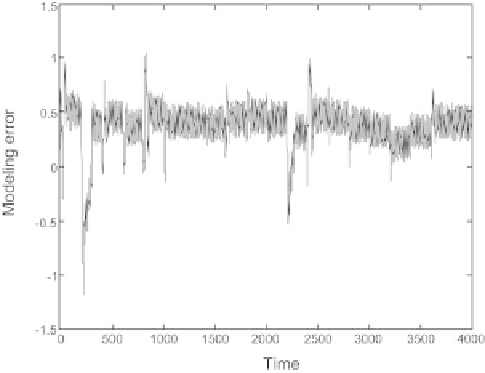
Fig. 2.52. Modeling error of the knowledge-based model

[ f [( k +1) T ] f ( kT )] /T (where k is a positive integer). Thus the following

discrete-time model is obtained:

−

x 1 [( k +1) T ]= x 1 ( kT )+ T [ − ( x 1 ( kT )+2 x 2 ( kT )) 2 + u ( kT )]
x 2 [( k +1) T ]= x 2 ( kT )+ T (8 . 32 x 1 ( kT )) .

Hence the simplest semiphysical model:

( x 1 ( kT )+2 x 2 ( kT )) 2 + u ( kT )]
x 2 [( k +1) T ]= x 2 ( kT )+ T ( wx 1 ( kT )) .

x 1 [( k +1) T ]= x 1 ( kT )+ T [ −

where w is a parameter that is estimated through appropriate training from
experimental data. The equations are under the conventional form of a state-
space model: it is therefore not necessary to cast the model into a canonical
form; were that not the case, the model would have been cast into a canonical
form as explained above. The model is shown on Fig. 2.53.
For simplicity, in all the following figures, the constant input (bias) will
not be shown; furthermore, discrete time kT will be simply denoted by k . q − 1
is the usual symbol for a unit time delay. On Fig. 2.53, neuron 1 performs a
weighted sum s of x 1 and x 2 , with the weights indicated on the figure, followed
by the nonlinearity −s 2 , and adds u ( k ). Neuron 2 multiplies its input by the
weight w . Neurons 3 and 4 just perform weighted sums. If w is taken equal
to 8.32, then this network gives exactly the same results as the numerical
integration of the discrete-time knowledge-based model by Euler's explicit
discretization, with integration step T .If w is an adjustable weight, then its
value can be computed by training the network from experimental data with
any good training algorithm (evaluation of the gradient of the quadratic cost
function by backpropagation through time, and gradient descent with the