Modeling with Neural Networks: Principles and Model Design Methodology - Neural Networks: Methodology and Applications - page 147

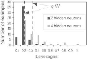
Fig. 2.27. Histogram of leverages for the best model with 2-hidden neurons and for
the best model with 4 hidden neurons

Thus, µ is a normalized quantity that may characterize of the leverage distri-
bution: the closer µ to 1, the more peaked the leverage distribution around
q/N . Thus, among models of different complexities having virtual leave-one-
out scores on the same order of magnitude, the model whose µ is closest to 1
will be favored.
We illustrate the usefulness of µ on the previous example. A test set of
N G = 100 examples was generated. The generalization error of the candidate
models can be estimated by computing the mean square difference between
the expectation value of the quantity to be modeled (which, in the present
academic example, is known to be sin x/x ) and the prediction of the model,

N G

1
N G

g ( x k , y )) 2 .

E G = ( E Y ( x k ) −

k =1

Figure 2.28 shows the quantities E p ,E T ,E G and µ , as a function of model
complexity. µ goes through a maximum that is very close to 1 for two hidden
neurons; that is the architecture for which the generalization error E G is
minimum. Thus, µ is a suitable criterion for a choice between models whose
virtual leave-one-out scores do not allow a safe discrimination.

Fig. 2.28. TMSE, virtual leave-one-out score, generalization error and µ , as a func-
tion of the number of hidden neurons