Modeling with Neural Networks: Principles and Model Design Methodology - Neural Networks: Methodology and Applications - page 100

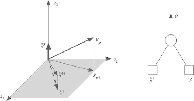
Fig. 2.3. Input orthogonalization by the Gram-Schmidt technique

ranking may be long or become numerically unstable for inputs that have very
small correlations to the output).
The procedure is illustrated on Fig. 2.3, in a very simple case where three
observations have been performed, for a model with two inputs (primary or
secondary) ξ 1 and ξ 2 : the three components of vector ξ 1 are the three mea-

sured values of variable ζ 1 during the three observations.
Assume that vector ξ 2 is the most correlated to vector y p . Therefore,
ξ 2 is selected, and ξ 1 and y p are orthogonalized with respect to ξ 2 ,which
yields vectors ξ 11 and y p 1 . If additional candidate inputs were present, the
procedure would be iterated in that new subspace until completion of the
procedure. The orthogonalization can be advantageously performed with the
modified Gram-Schmidt algorithm, as described for instance in [Bjorck 1967].

Input Selection in the Ranked List

Once the inputs (also called variables, or features) are ranked, selection must
take place. This is important, since keeping irrelevant variables is likely to be
detrimental to the performance of the model, and deleting relevant variables
may be just as bad.
The principle of the procedure is simple: a random variable, called “probe
feature” is appended to the list of candidate variables; that variable is ranked
just as the others, and the candidate variables that are less relevant than the
probe feature are discarded.
If the model were perfect, i.e., if an infinite number of measurements were
available, that input would have no influence on the model, i.e., training would
assign parameters equal to zero to that input. Since the amount of data is
finite, such is not the case.
Of course, the rank of the random feature itself is a random variable. The
decision thus taken must be considered in a statistical framework: there exists