Image Processing Reference
In-Depth Information
20
Nonlin. Local Models
Global Model
Eq. Constraints
Ineq. Constraints
20
Nonlin. Local Models
Global Model
Eq. Constraints
Ineq. Constraints
15
15
10
10
5
5
0
0
20
40
60
80
100
20
40
60
80
100
Frame #
Frame #
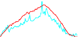
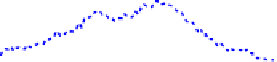
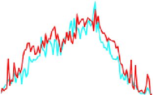
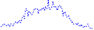
Figure 4.16:
Mean vertex-to-vertex distance between reconstructions and ground-truth meshes. The
reconstructions were obtained from synthetic correspondence (left) and SIFT correspondences (right).
Results were obtained with the linear local models of
Salzmann and Fua
[
2011
] with distance equalities
and inequalities, as well as with the nonlinear local models of
Salzmann
et al.
[
2008b
] (green) and the
global models of
Salzmann
et al.
[
2008a
] with distance equalities (cyan). The largest deformation appears
around frame 60, where the difference in accuracy is the greatest.
formulated as an SOCP problem by introducing slack variables
Boyd and Vandenberghe
[
2004
].
Doing so allows to re-write the problem as
c
+
r
−
λ
d
x
T
d
minimize
X
,
c
,
r
(4.17)
subject to
Mx
2
≤
c
,
(
x
−
x
0
)
2
≤
r
,
∀
(j, k)
∈
E
v
k
−
v
j
≤
l
j,k
,
,
which, like the problem of Eq.
4.4
, can be solved using a standard solver
Sturm
[
1999
]. As depicted by
Fig.
4.16
, the resulting solution of
Salzmann and Fua
[
2011
] tends to outperform the global smooth-
ness methods of
Salzmann
et al.
[
2008a
], as well as the nonlinear local models of
Salzmann
et al.
[
2008b
].
While the optimization problem of Eq.
4.16
is convex, it also is very large and takes a long
time to solve. As a result, this approach is ill-suited to real-time applications. One way to alleviate
this problem is to leverage the availability of a good initial solution to exploit efficient least-squares
resolution techniques. To this end, the problem of Eq.
4.16
can be reformulated as the constrained
least-squares minimization problem
2
2
minimize
X
Mx
+
(
x
−
x
0
)
(4.18)
subject to
v
k
−
v
j
=
l
j,k
,
∀
(j, k)
∈
E
.


Search WWH ::

Custom Search