Image Processing Reference
In-Depth Information
1400
1200
50
40
30
20
10
1000
800
600
400
0
180
190
200
210
220
230
240
250
260
200
0
0
50
100
150
200
250
300
(
(
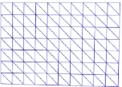
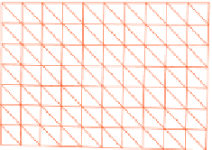
Figure 3.3:
Effective rank of matrix
M
. (a) 88-vertex mesh seen from the viewpoint used for reconstruc-
tion. (b) Singular values of
M
for the mesh of (a). Note how the values drop down after the 2
N
v
=
176
th
one. Although
M
was obtained with a full perspective model, this corresponds to the value predicted by
the weak perspective model of Section
3.3.1
. The small graph on the right is a magnified version of the
part of the graph containing the small singular values. The last one is zero up to the precision of the
Matlab routine used to compute it and the others are not very much larger.
(
(
(
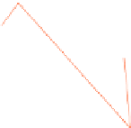
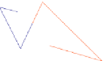
Figure 3.4:
Visualizing vectors associated to small singular values. (a) Reference mesh and mesh to which
one the vectors has been added seen from the original viewpoint, in which they are almost indistinguish-
able. (b) The same two meshes seen from a different viewpoint. (c) The reference mesh modified by
adding the vector associated to the zero singular value. Note that the resulting deformation corresponds
to a global scaling.
that the global scale is directly related to the position of the vertices along the lines of sight, which
produces one fewer small singular value.
The fact that the depth of the mesh vertices is ill-constrained shows that 3D-to-2D corre-
spondences on their own are not sufficient to reconstruct the shape of a surface from a monocular
image. Therefore, additional knowledge must be introduced in the problem. This can be done by
taking into account other sources of image information, such as shading. However, as mentioned


Search WWH ::

Custom Search