Database Reference
In-Depth Information
M
F
F
G
p
G
V
M
F
G
p
F
Ω
(
p
G
)
G
M
F
Ω
(
p
G
)
G
Ω
(
p
)
Ω
(
p
G
)
F
G
p
1
G
p
G
V
W
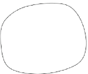
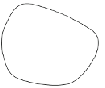
Fig. 4.5 Illustration of the stability of the mapping
M
F
. The first probability vector p
G
is inside
V
F
and modeled accurately by p
G
. The second probability vector p
G
is slightly outsi
de
V
F
and
modeled by the d
om
ain
p
G
which
is quite close to p
G
. The third vector p
G
is far from
V
F
leading to bad approximation results
(p
G
). Back
war
d transformation by F
G
leads to the domain
Ω
Ω
0
1
0
1
p
a
1
ss
1
p
a
2
ss
2
F
a
G
p
a
1
ss
1
0
1
@
A
p
a
1
ss
1
p
a
2
ss
2
p
a
3
ss
1
p
a
3
ss
2
@
A
p
a
1
ss
1
F
a
G
@
A
p
a
2
ss
2
p
a
1
ss
1
1
p
a
2
ss
2
þ p
a
1
ss
1
p
a
2
1
¼
¼
p
a
1
ss
1
þ p
a
2
ss
2
ss
2
F
a
G
p
a
1
p
a
2
ss
2
ss
1
;
p
a
2
ss
2
p
a
2
ss
2
1
p
a
1
ss
1
þ p
a
1
ss
1
p
a
2
F
a
G
p
a
1
p
a
2
ss
2
ss
1
;
p
a
1
ss
1
þ p
a
2
ss
2
ss
2
2
:
p
a
1
ss
1
p
a
2
ss
2
¼
F
G
1
can be derived. Here, F
a
G
¼
F
a
G
,
In the same way, the global mapping F
1
G
1
1
F
a
G
¼
F
a
G
, and F
a
G
is defined as F
1
according to (
4.7
). It is easy to see
that F
G
F
G
p
G
¼
p
G
W
.
However, since the space
V
consists of four free probabilities
p
a
1
8
p
G
∈
ss
1
,
p
a
2
ss
2
,
p
a
3
ss
1
,
p
a
3
ss
2
ss
2
1) and the space
W
only of the two
p
a
s
1
ss
1
,
p
a
s
2
(apart from the restriction
p
a
3
ss
1
þ p
a
3
ss
2
,
the image space
V
F
¼
F
G
(
W
) is really a proper subset of
V
, i.e., there exist
probabilities p
G
∈
V
: p
G
2 V
F
.
■
Thus, F
G
is really the inverse of F
G
. Since ran F
G
¼ V
F
V
is a proper subset
of
V
, the inverse F
1
G
is not defined over all elements of
V
. Unfortunately, our
observations are made in the space
V
. But technically, the mapping
M
F
defined by
Algorithm 4.2 can be applied to all vectors of
V
.
The good news is: since F
G
and F
G
are continuous and
V
,
W
are convex, as long
as ou
r a
ssumptions hold (Assumption 4.3 and the one of the nonlinear approach),
i.e., p
G
∈
V
F
, the result of the mapping
M
F
converges to the right solution
p
G
¼
F
G
p
ð
. If our assumptions are violated, i.e., p
G
2 V
F
, the r
es
ult of
M
F
is
oscillating. Yet, the second good news is: the closer the distance of p
G
to
V
F
, the
less is the oscillation. This is illustrated in Fig.
4.5
.