Database Reference
In-Depth Information
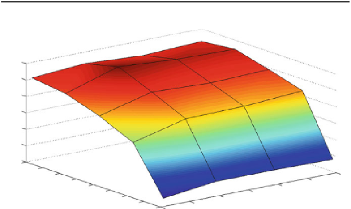
Table 9.2 Comparison of prediction rates (absolute): adaptive HOSVD with variable ranks
Rank w.r.t. the variation mode
Rank w.r.t. the master mode
10
100
200
300
10
48
56
56
55
100
104
120
121
126
200
122
139
136
138
300
136
156
151
149
400
141
146
142
145
160
140
120
100
80
60
40
400
350
300
300
250
250
200
200
150
150
100
100
50
50
00
Rang bzgi.des Master-Modes
Rang bzgi.des Variation-Modes
Fig. 9.4 Illustration of the prediction rates (absolute): adaptive HOSVD with variable ranks
The considered data set thus comprises 3,016 masters (i.e., products) and 596 var-
iations (i.e., colors). So, we would like the variation to act as another dimension. All in
all, we incorporate the master (dimension 1), the variation (dimension 2), and the
session (dimension 3). The factorization according to Algorithm 9.2 is carried out
on the training data, and we use the projection procedure (
9.5
) for the evaluation.
Thus, the employed method is consistent with that in the previous example with an
initial training set of 20,000 observations and a test set of 5,000 observations for the
actual evaluation.
Hence, on each product view, the slice
B
is formed as a matrix over all masters
and variations, whereupon we assign the value 1 to the hitherto considered prod-
ucts, i.e., their (master, variation) pairs, and 0 to the rest. We compute the updated
slice
B
t
by means of the projection procedure (
9.5
) and recommend the (master,
variation) pair with the highest value therein. After each session, we carry out an
incremental learning step with respect to all modes except the frontal one. This
corresponds to step 1 of Algorithm 9.2.
The result is displayed in Table
9.2
and in Fig.
9.4
.