Environmental Engineering Reference
In-Depth Information
When shifting
T
0
to the left/right on the horizontal axis, the curve
f
(
t
)
moves in the same direction without changing its shape. Thus,
T
0
is the
centre of dispersion of the random variable
T
, i.e. mathematical expectation.
The parameter
S
characterises the shape of the curve
f
(
t
), i.e. the
dispersion of the random variable
T
. As
S
decreases the p.d.f. curve
f
(
t
)
moves upwards and becomes sharper.
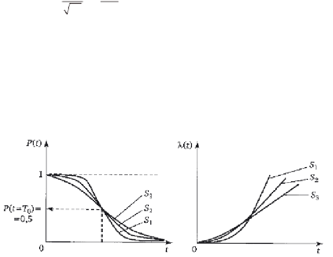
Changes of the graphs of
P
(
t
) and λ(
t
) at different standard deviations
of operating time (
S
1
<
S
2
<
S
3
) and
T
0
= const are shown in Fig. 1.15.
Using the previously obtained relations between the reliability indicators,
the expressions for
P
(
t
);
Q
(
t
) and λ(
t
) can be derived from the well known
expression [1.1] for
f
(
t
). It is clear that these integral equations are very
cumbersome and, therefore, the calculation of integrals for in practice is
replaced by tables.
To this end, we transfer from the random variable
T
to a certain random
variable
x tT S
= −
(
)/
,
[1.43]
0
distributed normally with parameters, respectively,
M
{
X
} = 0 and
S
=
{
X
} = 1 and the distribution density
1
−
x
2
[1.44]
fx
( )
=
exp
.
2
2
π
Expression [1.44] describes the density of the so-called normalised
normal distribution (Fig. 1.16).
The distribution function of random variable
X
is written in the form
x
=
∫
F x
()
f x dx
() ,
[1.45]
−∞
and the symmetry of the curve
f
(
x
) with respect to the EV
M
{
X
} = 0 shows
that
f
(-
x
) =
f
(
x
), from which
F
(-
x
) = 1 -
F
(
x
).
1. 15
Changes in graphs
P
(
t
) and
λ
(t) at different standard deviations
of operating time (
S
1
<
S
2
<
S
3
) and
T
0
= const.

Search WWH ::

Custom Search