Environmental Engineering Reference
In-Depth Information
∞
1
{
}
−=
∫
T
=
M T t
P t dt
() .
0|
tt
≤
1
Pt
()
1
t
1
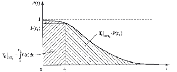
The relation between
TT
≤
,
tt
and
T
0
:
0|
0|
tt
>
1
1
T
+
T Pt
⋅
(
).
0|
tt
≤
0|
tt
>
1
1
1
T
>
are illustrated in Figure 1.6.
At the same time, the mean operating time can not fully characterise
the malfunction-free service of the object.
So, for the equal mean operating times to failure
T
0
the reliability of the
objects 1 and 2 can be quite significantly different (Fig. 1.7). Clearly, in
view of the large dispersion of operating time to failure (curve p.d.f.
f
2
(
t
)
below and wider), the object 2 is less reliable than the object 1.
Therefore, to assess the reliability of an object by value
T
0
it is necessary
to know and measure the dispersion of the random variable
T
={
t
}, near the
mean operating time
T
0
.
The dispersion indices include the
dispersion
and the
standard deviation
(SD)
of the operating time to failure
.
The dispersion of the random operating time
:
- statistical evaluation
The graphic concepts
T
and
0|
tt
≤
0|
tt
1
1
1
N
ˆ
ˆ
−
∑
2
D
=
(
t T
);
−
[1.39]
1
0
N
1
1
- probabilistic definition
∞
{ }
{
}
=−
∫
2
2
D D T M T T
= = −
(
)
(
t T f t dt
)
() .
[1.40]
0
0
0
The standard deviation of the random value of operating time:
ˆ
ˆ
ˆ
ˆ
{ }
{ }
2
2
2
S D S S T DT
=
or
=
.
=
[1.41]
The mean operating time to failure
T
0
and the standard deviation of
T
T
1. 6
Graphic concepts
≤
and
>
.
0|
tt
0|
tt
1
1

Search WWH ::

Custom Search