Environmental Engineering Reference
In-Depth Information
1. 2
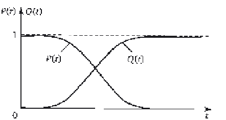
Graph of c.d.f. and FP.
It is obvious that the FP is a function of the distribution of
T
and
represents the probability that the time to failure is less than some specified
operating time
t
:
Q
(
t
) =
P
{
T
<
t
}.
[1.21]
The graphs of c.d.f. and FP are shown in Fig. 1.2.
In the limit as the number
N
(an increase of the sample) of test objects
increases,
P
(t) and
Q
(t) converge in probability (their values become
similar) to
P
(
t
) and
Q
(
t
).
Convergence in probability is as follows:
{
}
ˆ
P
lim| ()
Pt Pt
−
()| 0
==
1.
[1.22]
N
→∞
The determination of c.d.f. in the operating time range [
t, t
+ ∆
t
] is
of interest for practice, provided that the object had worked flawlessly
y to the beginning of the interval
t
. This probability is determined using
the multiplication theorem of probabilities and highlighting the following
events:
A
= {reliable operation of the object until the moment
t
};
B
= {reliable operation of the object in the range ∆
t
};
C
=
A·B
= {reliable operation of the object until the moment
t
+ ∆
t
}.
Obviously
P
(
C
) =
P
(
A·B
) =
P
(
A
)
·P
(
B|A
), since the events
A
and
B
are
dependent.
The conditional probability
P
(
B|A
) is c.d.f.
P
(
t, t +
∆
t
) in the interval
[
t, t +
∆
t
], so
P
(
B
|
A
) =
P
(
t
,
t
+ Δ
t
) =
P
(
C
)/
P
(
A
) =
P
(
t
+ Δ
t
)/
P
(
t
).
[1.23]
Failure probability in the operating time period [
t
,
t
+ Δ
t
], taking into
account [1.23], is:
Q
(
t
,
t
+ Δ
t
) = 1 -
P
(
t
,
t
+ Δ
t
) = [
P
(
t
) -
P
(
t
+ Δ
t
)]/
P
(
t
).
[1.24]
Statistical evaluation of the failure probability density function (p.d.f.)
is determined by the ratio of the number of objects ∆
n
(
t, t +
∆
t
), failed in
Search WWH ::

Custom Search