Physico–statistical models based on the residual defectiveness of structural materials - Probabilistic Safety Assessment for Optimum Nuclear Power Plant Life Management (PLiM) - page 175

N res ; N in ; N det , 1/mm

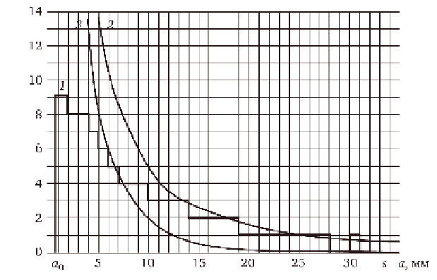
5.46 Histogram of defects detected in NDT and the envelope of
the defects 1; the curve of initial detectiveness 2; curve of residual
defectiveness 3.

Example 2

It is required to determine the probability of safe operation of pipelines
which can be in the 'leak before fracture' state.
There are 100 pipelines of the same type produced from seamless steel
pipes. In the welded joints distributed across the pipeline axis, ultrasonic
inspection prior to the start of service revealed technological defects
oriented in the transverse plane situated normal to the pipeline axis. The
defects were schematised by the same procedure as in the previous example
(Fig. 5.42).
The service life of the pipelines was 20 years. During this period, each
pipeline was subjected to 1500 internal pressure cycles.
Non-destructive inspection of all pipelines revealed a specific number of
crack-like defects in each pipeline. All the detected defects were schematised
by ellipses, and the minor semi-axis a = F / π c , where F is the area of the
defect, was determined for each ellipse.
The number of cracks of each standard size, detected in the 100
pipelines, was summed up and the mean value was determined:

￿ ￿ ￿ ￿ ￿

N det (χ) = N det.mean (χ) = [ N det1 (χ) + N det2 (χ) + N det3 (χ)+... N det100 (χ)]/100.

The average values of the number of the detected defects were used to
construct a histogram (Fig. 5.46, curve 1).
A test specimens with planar hidden defects was produced. The results
of inspection of the specimens were used to determine the reliability