Environmental Engineering Reference
In-Depth Information
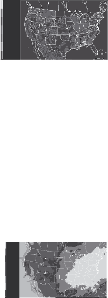
Simulations of toxaphene were
done for 18 months from 1 January
2000 to 30 June 2001 on the
domain shown in
Fig. 1
at a spatial
resolution of 36 × 36 km. In this
figure, the colour scale shows the
toxaphene emissions for the year
2000 calculated by the PEM emis-
sion model from residues that were
determined from the known toxa-
phene usage and an assumed soil
half-life of 4 years (James and
Hites, 2002). The residues were
allocated to the model domain using the gridded percentage of cropland (Envi-
ronment Canada, 2002) as a surrogate for spatial distribution.
2908.00 90
1000.00
100.00
10.00
1.00
0.10
0.01
0.00
1
kg/grid/yr
1
Fig. 1.
Toxaphene emissions for the year 2000 in the
model domain
3. Results and Discussion
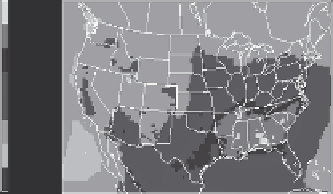
The simulated average surface gas
phase concentrations of toxaphene for
the year 2000 are shown in
Fig. 2.
The highest gas phase concentrations
coincide with the regions of highest
emission, but it is clear that they
extend into regions where there were
no residues and hence no emission.
(There are, for example, high gas
phase concentrations over the Atlantic
Ocean and the Gulf of Mexico.)
Because of the semi-volatile nature
of toxaphene, the surface gas phase
concentrations are dominated by
the emission, which is highest in the
summer. The transport, however, is
reflected by the spatial distributions
of deposition fluxes. The dry depo-
sitions are also dominated by the
surface concentrations, but deposi-
tions of particulate matter and wet
depositions are more dependent on
the meteorology.
1.0e-07 90
5.0e-08
1.0e-08
5.0e-09
2.0e-09
5.0e-10
1.0e-10
5.0e-11
1.8e-38
1
ppmV
1
132
Fig. 2
Gas phase toxaphene concentrations in the
lowest atmospheric layer (depth of 35 m)
4.5e-05 90
5.oe-06
1.oe-06
5.oe-07
1.oe-07
5.oe-08
1.oe-08
1.oe-11
1.8e-38
kg/hectare
1
132
Fig. 3
Averaged wet deposition of toxaphene
for the year 2002