Environmental Engineering Reference
In-Depth Information
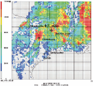
Fig. 1.
Isoprene emissions (mol/h) and the locations of power plants studied here
3. Results
The DI metric (Eq. 3) was computed for each power plant plume on each after-
noon at 2:00 pm. DI tended to be largest at the plants with the largest NO
x
emissions, likely reflecting a longer time for ozone to form as these more intense
plumes disperse. For most days of the episode, Martin Lake and Limestone were
the two power plants with largest DI and Parish had the smallest DI (
Table 1)
.
Table 1.
Locations, emission, electrical generation of power plants studied
Plant name
NO
x
emissions
(tons/day)
a
Annual electrical
generation (GWh)
b
Height of
stacks (m)
Distance of ozone
impact (km)
c
Deepwater
11.6
1,209
145
112
Limestone
40.9
13,017
137
140
Martin
48.5
17,239
137
138
Monticello
33.8
14,048
137
132
Parish
16.6
19,144
51-180
77
Welsh
26.9
10,395
92
107
a
c
From TCEQ, 2008. eGRID. At 2:00 pm
b
For each distance from each power plant, maximal ZOC
NOy
was used to diagnose
which cell was at the plume center. For large power plants, ozone production effi-
ciency tends to increase asymptotical with distance (a proxy for plume age) as the
plume dilutes and more ozone forms. The smaller power plants tended to reach
their maximal OPE at first due to more rapidly dilution to NO
x
limited conditions.
The nonlinearity index ( ) decreases dramatically with distance downwind of
the power plant, as the magnitude of
S
(2)
declines much more quickly than
S
(1)
(
Fig. 2)
. This is consistent with the findings of Cohan et al. (2005), who showed
that α increased with the intensity of a NO
x
plume.
α