Biomedical Engineering Reference
In-Depth Information
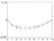
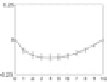
Figure 15.
Average subendocardial circumferential strain plots across 112 NURBS model
variants showing the mean (solid line) and standard deviation (error bars) for the predicted
strain values for the six basal (top row) and six mid-cavity (bottom row) regions.
The
dashed line represents the ground truth strain value predicted by the analytical model.
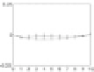
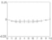
Figure 16.
Average subepicardial circumferential strain plots across 112 NURBS model
variants showing the mean (solid line) and standard deviation (error bars) for the predicted
strain values for the six basal (top row) and six mid-cavity (bottom row) regions.
The
dashed line represents the ground truth strain value predicted by the analytical model.
For all plots, end-diastole is assumed to occur at time
t
=0and is considered
the reference undeformed state for calculating Lagrangian strains. Since the plots
only demonstrate strain values during systole, peak strain is typically achieved
at the last time point shown. As compared with circumferential and longitudinal
directions, please note that there is a large variance in the radial direction for the
computed strains. This is likely due to lack of sufficient data points in the radial
direction.
6.2. In Vivo Canine Data: Left Ventricle
Assessment of our methodology for in vivo data incorporates both the residual
values from the least-squares fitting (e.g., Eq. (14)) as well as the average Jacobian
of the model. For subsequent analysis, we only show the residuals for the Eulerian
fits since those fits involve the data derived directly from the images (i.e., Eqs. (30),
(31), and (32)). Additionally, the Jacobian plots are derived from the Lagrangian
fits since we illustrate the capability of our model by plotting the Lagrangian
strains. The only exception is the case of the normal human volunteer for which