Biomedical Engineering Reference
In-Depth Information
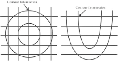
(a) Short-axis measurements (b) Long-axis measurements
Figure 8.
Diagrammatic representation of additional measurements for model fitting con-
sisting of the contour intersection points in the short- and long-axis views.
Each triplet of the lofted B-spline short- and long-axis tag plane surfaces
intersects at a single point. True displacement is available from the tracking of
each of these intersection points. This set of measurements is denoted as
M
I
=
{
p
i
+
d
i
}
,
(31)
where
d
i
is the true
displacement for the
i
th sample point at time
t
=0. The tag plane intersections
are calculated using the conjugate gradient descent algorithm [27].
The third set of measurements consists of the set of contour/tag line intersec-
tion points that provide displacement information along the epicardial and endo-
cardial surfaces of the model (Figure 8), defined by
p
i
is the position of an intersection point at
t>
0, and
M
C
=
{
p
i
+
v
i
}
,
(32)
where
p
i
is the position of the contour/tag line intersection point at
t>
0, and
v
i
is the component of the true displacement within the image plane for the
i
th
sample point at time
t
=0. The contour/tag line intersection points are calculated
using the conjugate gradient descent algorithm.
In addition to knowledge of the absolute position of the sample points, least-
squares fitting of B-splines also requires assigning parametric values to each sample
point. Due to the mapping explained previously, each measurement value,
m
i
,is
assigned the identical parametric vector, (
u
i
,v
i
,w
i
), as the origination point,
p
i
.
These parametric vectors are calculated from the NURBS model at time
t>
0 via
conjugate gradient descent. The coordinates of the position of the measurement
points contained in the sets
M
T
,
M
I
, and
M
C
for each time frame compose
the diagonal matrices
Ω
t
. Their corresponding parametric vectors
are used to formulate the observation matrices
Γ
t
,
Π
t
, and
B
γ
,
B
π
, and
B
ω
. For fitting the