Biomedical Engineering Reference
In-Depth Information
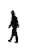
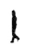
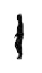
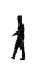
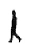
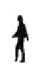
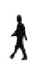
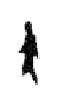
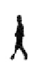
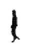
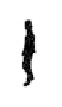
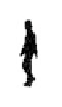
Sample training shapes
Isodensity
Sampling along geodesic (uniform dens.) Sampling along geodesic (kernel dens.)
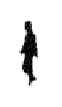
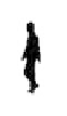
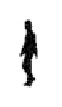
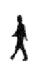
Figure 3.
Linear versus nonlinear shape interpolation. The upper row shows 6 out of 49
training shapes and a 3D projection of the isosurface of the estimated (48-dimensional)
shape distribution. The latter is clearly neither uniform nor Gaussian. The bottom row
shows a morphing between two sample shapes along geodesics induced by a uniform or
a kernel distribution. The uniform distribution induces a morphing where legs disappear
and reappear and where the arm motion is not captured. The nonlinear sampling provides
more realistic intermediate shapes. We chose human silhouettes because they exhibit more
pronounced shape variability than most medical structures we analyzed.
cian models. Second, in contrast to the joint estimation of intensity distributions
(cf. [15]), this simplifies the segmentation process, which no longer requires an
updating of intensity models. Moreover, we found the segmentation process to be
more robust to initialization in numerous experiments.
4.
ENERGY FORMULATION AND MINIMIZATION
Maximizing the posterior probability in (2), or equivalently minimizing its
negative logarithm, will generate the most probable segmentation of a given image.
With the nonparametric models for shape and intensity introduced above, this leads
to an energy of the form
E
(
α
,h,θ
)=
−
log
P
(
I
|
α
,h,θ
)
−
log
P
(
α
)
.
(7)
The nonparametric intensity model permits to express the first term, and equation
(6) gives exactly the second one. With the Heaviside step function
H
and the short
hand
H
φ
=
H
(
φ
α
,h,θ
(
x
)), we end up with
Nσ
.
K
α
−
α
i
σ
N
E
(
α
,h,θ
)=
−
H
φ
log
p
in
(
I
)+(1
−
H
φ
)log
p
out
(
I
)
dx
−
log
Ω
i
=1