Biomedical Engineering Reference
In-Depth Information
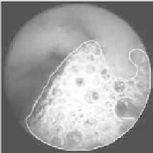
(a)
(b)
(c)
Figure 12.
Different results when changing the parameters controlling the smoothness of
the model: (a) rough model; (b) average smooth model; (c) smooth model. See attached
CD for color version.
subsection shows experiments designed to compare other deformable models with
the STOP and GO snake. Finally, the third subsection shows the application of this
deformable model to different domains and spaces in medical image processing.
6.1. Behavior of the STOP and GO Models
In this section we provide several experiments showing the behavior of the
STOP and GO active models. The first experiment shows how we can change the
degree of smoothness of the final model.
Figure 12 shows the results of changing the parameters governing the smooth-
ness of the model. In order to do so we just have to decrease the value of parameter
V
0
and the time increment ∆
t
. Note that for convergence issues around using this
numerical scheme, the condition
α
≤
0
.
4 must hold. As we can see, we can
obtain very smooth results; in particular, in [8] we show that the smoothness ob-
tained using these models is greater than that using classical deformable models.
This is due to the fact that we have two terms competing: on one hand, the cur-
vature term that tries to shrink the model; on the other, an area term repulsing the
model. Typical values for very smooth results are
α
=0
.
75, ∆
t
=0
.
5,
V
0
=0
.
5.
Figure 13 displays the number of iterations needed to obtain different degrees
of smoothness. As we can observe, there is a trade-off between the number of
iterations and the degree of smoothness. We need more iterations to create a
smoother model.
The final experiment of the STOP and GO behavior reflects control of the
·
∆
t
model for leaking through small gaps. Figure 14a shows the original image.
Figure 14b displays a co-occurrence feature space map where the deformable
model will evolve. Figures 14c,d show the final segmentation controlling leakage
through small holes. Figure 14c is obtained if we increase the value of
V
0
to force
the model to get inside the concave region. Figure 14d uses small values for
V
0
.